The distances to Novae as seen by Gaia

Louisiana State University Louisiana State University

LSU Scholarly Repository LSU Scholarly Repository

Faculty Publications Department of Physics & Astronomy

12-11-2018

The distances to Novae as seen by Gaia The distances to Novae as seen by Gaia

Bradley E. Schaefer

Louisiana State University

Follow this and additional works at: https://repository.lsu.edu/physics_astronomy_pubs

Recommended Citation Recommended Citation

Schaefer, B. (2018). The distances to Novae as seen by Gaia.

Monthly Notices of the Royal Astronomical

Society, 481

(3), 3033-3051. https://doi.org/10.1093/mnras/sty2388

This Article is brought to you for free and open access by the Department of Physics & Astronomy at LSU Scholarly

Repository. It has been accepted for inclusion in Faculty Publications by an authorized administrator of LSU

Scholarly Repository. For more information, please contact [email protected].

MNRAS 000, 1–17 (2018) Preprint 5 September 2018 Compiled using MNRAS L

X style ﬁle v3.0

The Distances to Novae As Seen By Gaia

Bradley E. Schaefer

Department of Physics and Astronomy, Louisiana State University, Baton Rouge, Louisiana, 70820, USA

Accepted XXX. Received YYY; in original form ZZZ

ABSTRACT

The Gaia spacecraft has just released a large set of parallaxes, including 41 novae

for which the fractional error is <30%. I have used these to evaluate the accuracy

and bias of the many prior methods for getting nova-distances. The best of the prior

methods is the geometrical parallaxes from HST for just four novae, although the real

error bars are 3× larger than stated. The canonical method for prior nova-distances has

b een the expansion parallaxes from the nova shells, but this method is found to have

real 1-sigma uncertainty of 0.95 mag in the distance modulus, and the prior quoted

error bars are on average 3.6× worse than advertised. The many variations on the

‘maximum-magnitude-rate-of-decline’ (MMRD) relation are all found to be poor, too

p oor to be useable, and even to be non-applicable for 5-out-of-7 samples of nova, so

the MMRD should no longer be used. The prior method of using various measures of

the extinction from the interstellar medium have been notoriously bad, but now a new

version by

Ozd

onmez and coworkers has improved this to an unbiased method with

1-sigma uncertainty of 1.14 mag in the distance mo dulus. For the future, I recommend

in order (1) using the Gaia parallax, (2) using the catalog of

Ozd

onmez, (3) using

m ax

= -7.0±1.4 mag as an empirical method of poor accuracy, and (4) if none of

these methods is available, then to not use the nova for purposes where a distance is

needed.

Key words: parallaxes – stars: novae, cataclysmic variables

1 INTRODUCTION

A ubiquitous and deep problem of high importance through-

out the last century of astrophysics has been measuring the

distances to objects. Realistic distances are critical to un-

derstanding the structure and organization of the objects,

while the inverse-square dependency of the luminosities and

energies on the distances means that any physical model

must have good distances. For novae, the last century has

also featured much eﬀort and debate to get distances.

Many methods have been used to estimate nova dis-

tances. With geometrical parallaxes ($) not possible (ex-

cept for four of the nearest novae as viewed with the Hubble

Space Telescope, HST), the standard has been to use ex-

pansion parallaxes for the few novae with shells. But even

this standard was known to be poor for multiple reasons,

and it could not be applied to most novae. For most novae,

with no other possibilities, workers could only make order-

of-magnitude distance estimates based on various measures

of the interstellar extinction, with such methods being no-

toriously poor. (But

Ozd

onmez and coworkers have recently

E-mail: [email protected]u

found ways to make this work, see below.) With these poor

calibrations, workers attempted to ﬁnd a relation between

the nova’s absolute magnitude at peak and the speed of de-

cline (called the ‘maximum-magnitude-rate-of-decline’ rela-

tion, or the ’MMRD’). But this correlation has a huge scatter

making the method largely useless, while recently the very

existence of the relation has been disproven for novae in M31

and M87. Another method from the past few years has been

to get blackbody distances to the secondary stars. But this

method is untested, and is applicable to only a half-dozen or

so systems. So in all, until now, the all-important distances

to novae are poorly known.

Now, with the public release of many accurate paral-

laxes from the Gaia spacecraft, we ﬁnally have conﬁdent and

accurate distances to many novae. Suddenly, we can evalu-

ate all the prior nova distances and their methods. This has

vital relevance for future nova studies because Gaia will only

get good parallaxes for less than 20% of the known novae.

For the other 80%, we still have to rely on the many other

methods, so it is good to learn the real accuracy and biases

of each method. Thus, a primary purpose of this paper is to

evaluate the prior published nova distances as based on the

Gaia ‘ground-truth’.

arXiv:1809.00180v1 [astro-ph.SR] 1 Sep 2018

2 B. E. Schaefer

2 OBSERVATIONS

The European Space Agency Gaia satellite is awesome in its

capabilities for astrometry, for getting parallax and proper

motions of stars far out into our Milky Way galaxy. The sec-

ond data release (DR2) has just come out, with 22 months of

operational data covering 1693 million stars from magnitude

3 to 21 (Lindegren et al. 2018). DR2 is publicly available

on-line

. DR2 includes positions, proper motions, and paral-

laxes (ﬁve astrometric parameters), with all sources treated

as single stars. No binary motion or source confusion is al-

lowed for, with these being covered in later data releases.

The distribution of errors in the parallax is essentially a

perfect Gaussian with the quoted 1-sigma error bars (Luri

et al. 2018). The standard uncertainty for $ is 0.041 milli-

arc-seconds (mas) for 12 mag stars, 0.057 mas for 16 mag

stars, and 0.651 mas for 20 mag stars.

The traditional equation to derive the distance, D in

parsecs, from the observed parallax, $ in mas, is D =

1000/$. But various workers have long realized that the

conversion from parallax to distance is really much more

complex and subtle. The trouble comes when the observed

parallax is small when compared to its uncertainty. At its

extreme, a zero parallax would translate to an inﬁnite D,

with this being unphysical, while a perfectly good negative

parallax is meaningless. A common problem is that the un-

certainty in distance will have a substantially non-Gaussian

shape, with the distribution being greatly skewed when the

uncertainty in the parallax, σ

, grows to a substantial frac-

tion of the parallax. For example, with an observed parallax

of 0.5±0.5 mas, the 1-sigma range in parallax is 0.0 to 1.0

mas, yet the same 1-sigma range in distance is from 1000

pc out to inﬁnity. And the simple equation does not tell

us how to handle the negative part of the parallax’s distri-

bution. These problems become non-trivial for cases where

/$&20% or so (Bailer-Jones 2015).

The solution to the inversion problem (i.e., to go from

a measured parallax to the best distance with realistic error

bars) is now know to require some appropriate assumption

about the distance distribution, known as a ‘prior’, within a

Bayesian analysis. An excellent explanation and tutorial is

presented in Bailer-Jones (2015). The solution is to adopt a

prior where the a priori probability volume density decreases

asymptotically to zero at inﬁnity. A reasonable function for

the prior is an exponential decline with some appropriate

distance scale. The oﬃcial Gaia DR2 publication (Luri et

al. 2018) explicitly endorses this ‘exponentially decreasing

space density’ (EDSD). With this, the probability distribu-

tion of D is given by equation 18 of Bailer-Jones (2015), and

I have performed the integrals on this unnormalized poste-

rior to deﬁne the 1-sigma intervals containing the central

68.3% probability. The best estimate distance is given by

equation 19 of Bailer-Jones. When σ

/$ rises above 0.30,

two modes appear in the posterior, one of which is ‘data-

dominated’ and the longer distance is ‘prior-dominated’, so

by the time the fractional error rises above 0.373 there is a

sudden increase in the mode.

So, given the Gaia values for $ and σ

along with the

EDSD, the only question is the appropriate length scale.

Here I have taken the length scale to be 150/sin(l) parsecs,

https://archives.esac.esa.int/gaia

with a maximum of 8000 pc, where l is the galactic latitude,

for a disk population. For a halo population, I adopt a length

scale of 8000 pc.

Let us see how all this works for some schematic cases:

For a case with a length scale of 1000 pc, a measured par-

allax of 10.0±0.1 mas gives a D with 1-sigma error bars of

100

−1

pc, 1.0±0.1 mas gives 1010

+142

−76

pc, 0.1±0.1 mas gives

4600

+2300

−730

pc, and -0.1±0.1 mas gives 6200

+2700

−1050

pc. For a case

with a length scale of 8000 pc, 10.0±0.1 mas gives 100

−1

pc,

1.0±0.1 mas gives 1019

+147

−77

pc, 0.1±0.1 mas gives 14300

+21100

−3300

pc, and -0.1±0.1 mas gives 21500

+21000

−5300

pc.

The Gaia Data Release 1 (DR1) has already returned

the parallaxes for three novae (V603 Aql, RR Pic, and HR

Del), as based on comparisons of Tycho positions plus early-

epoch Gaia positions (Ramsay et al. 2017). But these early

DR1 results have quoted error bars over a full order-of-

magnitude larger than the DR2 results. Nevertheless, the

Ramsay et al. study provided the ﬁrst look at nova-distances

with Gaia, showing that the short distance scale to SS Cyg

was correct, and providing the ﬁrst indications that the prior

HST parallaxes and the expansion parallaxes were greatly

worse than advertised.

I have examined 120 novae for reliable inclusion in the

Gaia DR2 data base. A total of 64 novae are included in

Table 1. These are divided into three samples, which I label

as the ‘Gold’, ‘Silver’, and ‘Bronze’ samples. The 26 Gold

novae are those with very well observed light curves from

the SSH sample (Strope, Schaefer, & Henden 2010; SSH) for

which Gaia has a conﬁdent detection and a parallax with less

than 30% error. The SSH sample of novae contains the 93

all-time best observed nova light curves, all with exhaustive

light curve information collected together and systematically

analyzed for the various needed light curve properties. The

Gold sample is the best and most reliable, mainly because

these novae are generally the nearest and brightest. The 15

Silver novae are mostly well observed events which are not

included in SSH for various reasons, and for which Gaia

returns a conﬁdent identiﬁcation with a parallax error of

<30%. The 41 novae in the Gold+Silver sample comprises

all the conﬁdent and accurate novae parallaxes, and this is

my basic group for testing the prior distances. The 23 Bronze

novae are those for which there is a reliable Gaia detection,

but for which the quoted parallax error bar is >30%. These

novae have no real utility for testing prior distance measures.

However, there is information in the Gaia parallax measures,

but only for statistical purposes.

Many novae are not included into Table 1, for many

reasons. Three recurrent novae with red giant companion

stars (T CrB, RS Oph, and V3890 Sgr) do not have reliable

Gaia parallaxes because their long-period binary orbits will

cause the center-of-light to wobble with shifts comparable to

the parallaxes, so we must await a full solution with a later

data release. The unique nova V445 Pup is recognized in the

DR2 catalog, but no parallax is recorded. Eleven old novae

(including DO Aql, V5592 Sgr, and V1213 Cen) have more

than one candidate around the correct position, but I cannot

decide with any useable conﬁdence as to which (if any) DR2

objects are the real quiescent counterparts. Twenty-six old

novae (including V2274, V2362, and V2467 Cyg, plus V2264,

V2295, V2313, and V2540 Oph) have no conﬁdently identi-

ﬁed counterpart (often likely because the counterpart is very

MNRAS 000, 1–17 (2018)

Nova Distances With Gaia DR2 3

faint) so no DR2 object can be taken as a reliable counter-

part. Fifteen old novae (including Nova Sco 1437, V728 Sco,

V977 Sco, and V1187 Sco) have counterparts that are not

seen by Gaia.

For possible inclusion in Table 1, I have looked at nearly

all the known galactic novae for which even poor light curves

are available and for which a counterpart is known. For the

galactic novae with a conﬁdent counterpart in Gaia DR2

with σ

/$ < 30%, that is the Gold and Silver samples, I

think that Table 1 is complete. For the galactic novae with a

conﬁdent counterpart with σ

/$ > 30%, that is the Bronze

sample, I think that Table 1 is nearly complete, while pos-

sibly missing some obscure novae.

I have included in the Silver sample two unexpected

nova, both being well-known cataclysmic variable (CV) sys-

tems with dwarf nova (DN) eruptions. Both Z Cam and AT

Cnc were discovered to have expanding nova shells pointing

with conﬁdence to classical nova eruptions within previous

centuries, plus the historical identiﬁcation of ‘guest stars’ in

ancient chronicles (Shara et al. 2007; 2012a; 2016). There

is little light curve information for these old novae. Still,

they are useful because they represent two more cases for

the small set of systems with observed classical nova (CN)

eruptions as well as DN, and these nova systems now have

reliable distances and absolute magnitudes in quiescence,

with application to testing the ‘hibernation model’ (Shara

et al. 1986) of CV evolution.

Table 1 lists all the novae in the Gold, Silver, and Bronze

samples, plus many properties for each nova. My primary

reference is my nova light curve catalog (Strope, Schaefer,

& Henden 2010, SSH), as this contains a comprehensive

and uniform measure of all light curve information for the

93 best-observed novae of all time. This is exactly what is

needed for many of the tests of prior distance measures.

Other primary reference sources are Schaefer (2010) for re-

current novae (RN), Schaefer & Patterson (1983) for BT

Mon, Schaefer et al. (2013) for T Pyx, Salazar et al. (2017)

for V1017 Sgr, Schaefer & Collazzi (2010) for the V1500

Cyg class of novae, and Pagnotta & Schaefer (2014) for

many light curves and properties. Further primary reference

sources as compilations of many nova properties include the

three wonderful and comprehensive papers of Shafter (1997),

Duerbeck (1981), and

Ozd

onmez et al. (2018), plus the on-

line CV Catalog of Downes, Webbink, & Shara (1997). For

light curve information, for example for the recent nova V392

Per, I have made extensive use of the light curves of the

American Association of Variable Star Observers (AAVSO).

For particular novae where there is some gap in the infor-

mation, or where the sources put forth conﬂicting values, I

have extensively consulted the original papers with the ob-

servations.

In Table 1, column 1 lists the nova. Column 2 lists the

sample, either Gold, Silver, or Bronze. Column 3 gives the

nova type, with the basic division being the ‘classical novae’

(CN) and the ‘recurrent novae’ (RN). Various additional di-

visions are included, for example the notation ‘DN’ indicates

that the nova system has been seen to experience dwarf nova

eruptions. (To anticipate, these novae are indistinguishable

from the other novae in terms of their absolute magnitude

in quiescence, with this violating a prediction of the ‘hiber-

nation model’ for the evolution of CVs.) ‘Hi-∆m’ notates

that the star is a V1500 Cyg system, where the long-post-

eruption quiescence magnitude is over 2.5 mag brighter than

the pre-eruption magnitude (Schaefer & Collazzi 2010). (To

anticipate, what I will ﬁnd is that the V1500 Cyg systems

are greatly less luminous in quiescence than all other no-

vae systems.) I also notate for V838 Her that it has been

identiﬁed by Pagnotta & Schaefer (2014) as being a likely

RN that has had multiple eruptions in the last century but

with only one such discovered. Further, I note that AR Cir

might be a symbiotic system (i.e., have a red giant compan-

ion star), and might have had a symbiotic nova eruption.

Column 5 completes the block describing the novae by giv-

ing the light curve classiﬁcation from SSH. ‘S’ denotes no-

vae with a smooth light curve, ‘P’ is for light curves with

distinct plateau around the transition phase, ‘O’ class novae

show quasi-periodic oscillations around the transition phase,

‘D’ novae are those with a deep dust dip in the light curve,

‘F’ novae display a long ﬂat top at the maximum of their

light curve, ‘J’ novae have large ﬂares or jitters in their light

curve around the time of maximum, and ‘C’ novae have a

distinct cusp with a slow and accelerating rise to a second

maximum followed by a fast fall.

The next block of Table 1, columns 6 and 7, give the new

Gaia input. This is the measured parallax and its 1-sigma

error bar (in units of milli-arcseconds), and the derived dis-

tance (in units of parsecs). Again, the distances are derived

with the EDSD Bayesian prior, and the quoted error bars

display the central 68.3% of the probability distribution.

The next block of Table 1 contains 6 columns with light

curve information. Column 8 reports the peak magnitude,

m ax

. For two systems (Z Cam and AT Cnc) for which the

nova is only known from ancient historical records (as well as

from their expanding shells), the peak is not known, but it

must have been something like 0±3 mag. It is diﬃcult to de-

ﬁne a formal error bar even for the well-observed light curves

from SSH, but a typical real uncertainty is roughly 0.1–0.2

mag. Some of the light curves in the Silver and Bronze sam-

ples are poorly sampled and the real error bars for V

m ax

can be more like 0.2–0.5 mag. For V1017 Sgr and CT Ser,

the peaks were apparently missed, so there is large uncer-

tainty in V

m ax

, as indicated in column 8. Column 9 gives the

magnitude at a time 15 days after peak, V

15d

, and the uncer-

tainties are only larger than for V

m ax

. An additional problem

is knowing the date of the peak (especially in the case of the

J-class novae), and often the light curve 15-days after the

maximum is fast fading, so large changes in V

15d

result from

modest uncertainties in the peak date. Column 10 gives the

average quiescent magnitude, V

. I have taken pre-eruption

magnitudes (Collazzi et al. 2009) in preference when avail-

able. (This is important for the V1500 Cyg stars, as the

absolute magnitude before eruption is better to show the

accretion rate appropriate for the long-term evolution.) The

ubiquitous magnitude variations in quiescence are roughly

0.5–2.0 mag, so with the inevitable poor sampling, it will

be hard even to deﬁne the average with much accuracy. The

uncertainties in V

are hard to know, although typical error

bars might be ±1 mag. Column 11 is the V-band extinction

) from the interstellar medium. Most of the tabulated ex-

tinctions are from compilations involving multiple measures

from a wide variety of methods. I have converted reported

E(B − V) values to A

as 3.1 × E(B − V), as appropriate for

the local dust in our Milky Way’s disk. Again, formal error

bars for extinctions are hard to get, with typical uncertain-

MNRAS 000, 1–17 (2018)

4 B. E. Schaefer

ties being perhaps 0.1–0.3 or perhaps 10%–30%. Columns

12 and 13 list the values for t

and t

, given in units of days,

deﬁned as the time it takes the light curves to fall by 2.0

or 3.0, respectively, mag from the peak. Again, formal error

bars are diﬃcult, even for well-sampled S-class light curves,

and real error bars might be 10%–30%. For novae with sub-

stantial jitters or with poorly sampled light curves, the real

error bars can easily be 30%–50%.

The last block of Table 1 is the derived absolute mag-

nitudes at maximum (M

m ax

) and in quiescence (M

). These

are calculated from the tabulated values with the absolute

magnitude equalling V − A

− 5 log[D] + 5.

3 TESTING PRIOR DISTANCES TO NOVAE

For comparing the prior nova-distances with those from

Gaia, we need quantitative measures of the errors in the dis-

tance. The size the distance errors can be quantiﬁed as some

function of either D

pr ior

− D

Gaia

= ∆D or D

pr ior

Gaia

where D

pr ior

is the pre-Gaia distance from a set being

tested in this paper and D

Gaia

is the distance from the

Gaia parallaxes. The errors in these will be dominated by

the prior measures, and these are often with asymmetrical

distributions, such that the quantity log

pr ior

Gaia

]

will usually have a more symmetric distribution. With a

common use for the nova distances being to get luminosi-

ties and energetics, a useful measure of the distance error

will be the error in the distance modulus, ∆µ. We have

∆µ = 5 × log

pr ior

Gaia

]. This quantity tells us the

error in the absolute magnitude arising due to the error in

the prior distance to the nova. This can be related to the

fractional distance error as F = ∆D/D

Gaia

= 10

∆µ/5

− 1.

The F value loses its simple meaning as a symmetric mea-

sure when F starts getting large, so the ∆µ statistic is the

general solution.

With multiple independent measures of ∆µ for a set of

prior nova distances, the RMS scatter will equal the average

measurement error for the set. Note, this RMS scatter will

be about some best ﬁt average, so that if the prior distances

have a substantial bias, the real errors in the prior distances

will be substantially larger. In general, the bulk of this scat-

ter in ∆µ comes from the uncertainty in the prior distance, so

we can adopt the RMS scatter, σ

∆µ

as the easy-to-calculate

measure of the 1-sigma error bar for the average of the prior

distances. The prior distances might be biased, either long

or short. This can be quantiﬁed by the average diﬀerences

in the distance moduli, h∆µi.

We also need a measure of the size of the error bars

for the prior distances. I will use the measure χ ≡ ∆D/σ,

with a similarity of meaning as in the usual chi-square

summation. The total error bar in the diﬀerence ∆D is

= σ

pr i or

+ σ

G ai a

. If the quoted error bars are ac-

curate, then the distribution of the observed χ values for a

set of nova distances should have an RMS scatter of near

unity. If the error bars are systematically smaller than the

real scatter in the distance errors, then the RMS will be

much larger than unity. So σ

is a measure of the relative

size of the quoted error bars with respect to the real error

bars.

Of the various possible measures of the errors, individ-

ual novae can be quantiﬁed with ∆ µ, while the average real

errors of the collection of distances can be represented by

∆µ

, the size of the reported error bars can be expressed by

, and the bias in the reported distances is h∆µi. An un-

biased set of prior distances with σ

=10% errors will have

∆µ

near 0.21 mag, σ

1.0, and h∆ µi0.0.

For some applications, it is useful to deﬁne similar

statistics involving the parallax itself (as opposed to the dis-

tance), with this enjoying the advantage that the error bars

in parallax have a good Gaussian distribution. The statis-

tic ∆µ = 5 × log

Gaia

pr ior

] can be easily calculated.

With this, we can get h∆µi and σ

∆µ

. We can also deﬁne the

fractional error in parallax as F = ($

pr ior

− $

Gaia

)/$

Gaia

with this being similar to F. As a measure of the size of the

error bars, we can use the statistic ψ ≡ ($

pr ior

−$

Gaia

)/σ

with σ

= σ

pr i or

+ σ

G ai a

. The RMS value of ψ for a set

of novae parallaxes will be σ

, with this being similar and

close to σ

. So the quality of a set of prior novae parallaxes

can be evaluated with the three values for h∆µi (a measure

of bias high-or-low), σ

∆µ

(measure of the real 1-sigma error

in the associated magnitude), and σ

(a measure of the size

of the reported error bars).

In this section, I will systematically check prior nova

distances from many diﬀerent methods. I will not address

the important sets of novae that reside in other galaxies

(LMC, M31, and M87) for which many workers have derived

distances independent of the novae.

3.1 Testing Prior Parallaxes

For the past history of astronomy, the geometrical parallax

has always been the ‘gold standard’. Unfortunately, few no-

vae can get any useable parallax, at least before Gaia. The

only prior useable parallaxes were measured with the Fine

Guidance Sensors, FGS, on the HST (Benedict, McArthur,

Nelan, & Harrison 2016). Harrison et al. (2013) report on

FGS parallaxes for four of the brightest and nearest classi-

cal novae.

The FGS measured parallaxes are given in Table 2 and

Figure1, along with the measured parallaxes of Gaia DR2.

I will make the comparison between the parallaxes (and not

the derived distances) because that is possible for the FGS

parallaxes without any conversions dependent on Bayesian

priors, and then the quoted error bars will have a Gaussian

distribution.

In a comparison of the HST and Gaia parallaxes, we

see a relatively good match. However, the diﬀerences are

large compared to the claimed error bars. The worst case

is for V603 Aql, where the diﬀerence in reported parallaxes

is 0.820 mas, while the total 1-sigma uncertainty in the dif-

ference is 0.153 mas, so the HST parallax is in error by

ψ=5.4-sigma. This is too large to be from random measure-

ment error with the quoted error bars. And the parallaxes

for DQ Her are diﬀerent at the ψ=2.9-sigma level. This again

suggests that the HST parallaxes have some unrealized and

substantial systematic error. Both of these cases have the

HST parallaxes being larger than the Gaia values. However,

GK Per has a ψ=-1.3-sigma deviation, while RR Pic has a

ψ=-0.2-sigma deviation, both in the opposite direction from

the ﬁrst two, with these two cases showing scatter as might

be expected from random measurement errors. So we have a

mixed bag for the comparisons, with half the novae having

MNRAS 000, 1–17 (2018)

Nova Distances With Gaia DR2 5

apparent signiﬁcant systematic errors, while the other half

does not.

To be quantitative, the average value of the diﬀerence

in the distance moduli is h∆µi = −0.21, while the RMS scat-

ter of these diﬀerences is σ

∆µ

= 0.37. This corresponds to

an RMS error in the parallax of 19%. The diﬀerences in

parallax, in units of the total 1-sigma error bar, has an aver-

age of hψi=1.7 and an RMS of σ

=3.03. This goes to show

that the FGS parallaxes have systematic errors that average

three-times larger than the quoted error bars. So the real

FGS error bars are on average 3× larger than published.

Unfortunately, the one other HST FGS parallax to a

CV also shows big problems. In particular, Harrison et al.

(1999; 2000; 2004) reported that the prototypical dwarf nova

SS Cyg has a parallax of 6.06±0.44 mas. But this was found

to disagree greatly from the VLBI measured parallax of

8.80±0.12 mas (Miller-Jones et al. 2013). Further, the small

reported FGS parallax forced SS Cyg to such a high lumi-

nosity such that accretion-disk theory strongly states that

the dwarf-nova-instability is impossible (Schreiber & La-

sota 2013). This set up a severe conundrum for the ﬁeld

of CVs (that includes novae). Most workers in our commu-

nity thought that the discrepancy was resolved by Nelan

& Bond (2013) when they did a complete reanalysis of the

same FGS data and derived a parallax of 8.30±0.41 mas.

Now, Gaia gives a parallax of $

Gaia

=8.724±0.049 mas, and

all doubts about the controversy are gone. So the conclu-

sion is that the early reported FGS parallax must have had

some sort of subtle analysis error. This is disconcerting be-

cause the Harrison papers had triply-repeated analysis by

the best and most experienced workers in both astrometry

and in the HST FGS. The lesson from this is that even the

HST FGS parallaxes are suﬃciently tricky as to have large

systematic errors.

This is all rather discouraging for the FGS parallaxes.

However, to keep the issues in perspective, the FGS nova

distances are still the best measures prior to Gaia.

To further evaluate geometrical parallaxes for CVs, we

have a long series of ground-based measures of very nearby

systems by J. Thorstensen and coworkers. In a tour de

force, Thorstensen (2003) and Thorstensen, L´epine, & Shara

(2008) present 26 geometrical parallaxes for faint and nearby

CVs, with the images taken with the 2.4-m telescope at

MDM Observatory. These can be compared to the Gaia DR2

parallaxes (see Figure1). I ﬁnd that the RMS scatter of the

diﬀerences in distance moduli is 0.54 mag, while the aver-

age diﬀerence is -0.37 mag. The diﬀerences in units of the

total 1-sigma diﬀerence have an RMS scatter of 1.06. With

this, we see that the Thorstensen parallaxes have an accu-

racy only slightly worse than HST, a moderate bias towards

overestimating the CV distances, and accurately reported

error bars. This reliability and accuracy is remarkably good.

3.2 Testing Expansion Parallaxes From Nova

Shells

Novae often eject visible shells, seen to expand for years

and decades. If we take the expansion velocity of some part

of the shell to be given by some part of the wings of the

early nova emission lines, then the distance to the nova is a

simple calculation from the angular size of the shell and the

time since the eruption. Such distances are called ‘expansion

parallaxes’. Such distances are known for only around 30

novae. In the absence of real parallaxes, these distances were

perceived as being the best around, and thus the expansion

parallaxes became the primary way to calibrate and test

other distance methods.

Unfortunately, this method has a greatly-larger real un-

certainty than is usually recognized. (1) The relevant veloc-

ity might be given by the Half-Width-Zero-Intensity or the

Half-Width-Half-Maximum of the emission line proﬁle, with

a factor of two diﬀerence in distance. And many novae have

weird ‘castellated’ proﬁles or P-Cygni proﬁles, and it is to-

tally unclear as to what to use then. Indeed, the literature

has little discussion and no understanding as to where to

pick the velocities from the proﬁles. Further, the proﬁles

vary substantially from line-to-line, and the line widths de-

crease by over factors of two from early-to-late in the erup-

tion. All of these lead to roughly factor-of-two errors in the

distances. (2) The relevant angular radius can be taken from

a wide range of isophotal values, from the peak of some sup-

posed ring, to the edge as deﬁned by the steepest drop in

the proﬁle, to the outermost position with shell light. Many

shells are poorly resolved, with some correction required for

the point-spread-function of the imaging, with few workers

making any such corrections. Most shells have large-scale

out-of-round shapes (with observed axial ratios up to 1.42,

see Downes & Duerbeck 2000), and have knobby features

that extend out farther, so which radius should be used?

For the ‘simple’ question of using just one (out of a contin-

uum) of isophotal levels, Wade et al. (2000) have six diﬀerent

ways of deﬁning the eﬀective radius. The literature has little

discussion and no theoretical guidance as to how to choose

a radius that corresponds to the velocity somehow selected.

Rather, multiple workers just plea for observers to simply

report what they did, a plea that is usually dodged. Again,

these reasonable choices lead to a factor of two uncertainty

in the distances. (3) The radial velocities along the line of

sight are usually substantially diﬀerent from the expansion

velocity in the transverse directions. This is demonstrated

by the fact that most novae have substantially out-of-round

shells (Downes & Duerbeck 2000). This is further shown for

many novae with massive high-velocity jets (e.g., GK Per,

see Shara et al. 2012b) and for shells with bipolar shapes.

For the third time, we recognize ubiquitous errors at the

factor-of-two level, with none of these being discussed much

or included in published error bars.

To test the expansion-parallax distances, I have col-

lected published values for 22 novae that are in my Gold and

Silver samples. Most of them have many published values,

with these being given in Table 3. These values have been

compiled from Downes & Duerbeck (2000),

Ozd

onmez et al.

(2016), Slavin (1997), and Shafter (1997), which are them-

selves compilations of values calculated from many sources.

The distances for each nova are not all independent, with

many of the results sharing input.

It is disconcerting to see the huge range of values for

many of the novae. This is a strong measure of the large size

of the real error bars for the expansion-parallax method.

Further, a third of the published distances have larger than

50% true errors. On the plus side, only 12% of the published

distances have errors by greater than a factor of two.

The ﬁrst set I will evaluate is the distances collected

in Slavin (1997), because this includes quoted error bars for

MNRAS 000, 1–17 (2018)

6 B. E. Schaefer

all. For this set of 9 novae, I calculate that σ

∆µ

equals 1.04

mag, corresponding to a 1-sigma uncertainty of a factor of

2.6× in luminosity. Further, σ

equals 3.6, which shows that

the reported error bars are on average a factor of 3.6× too

small. With h∆ µi= -0.10 mag, there is no bias.

The next data set is all 75 measures reported in Table

3 (see Figure 2). Most of these have no quoted error bars.

A measure of the real error in the reported distances is that

∆µ

= 0.95 mag, which points to an average 1-sigma error

of a factor of 2.4× in luminosity. The expansion-parallax

distances appear unbiased, as h∆µi equals -0.06 mag. For

use in calculating σ

, I have adopted σ

pr i or

= C × D

pr ior

as some sort of an average error. I must adjust C to equal

0.60 so as to get σ

equal to unity, which is to say that the

real error bars are 60% on average.

What we see is that the expansion-parallax method is

far worse than is the popular idea that this is the canoni-

cal method. (But I expect that the researchers who special-

ize in the method are well aware that the real uncertain-

ties are frustratingly large, c.f. Downes & Duerbeck 2000;

Wade, Harlow, & Ciardullo 2000.) The real error is some-

thing like 2.6×, and this makes this method largely use-

less for many applications. Still, for some applications, the

expansion-parallax is the best that we can get, and a factor-

of-two is better than no idea at all.

3.3 Testing Blackbody Distances For The

Secondary Stars

A relatively new method to get a distance to a nova is to

derive the blackbody distance to the secondary star. To do

this, we need to isolate the ﬂux from the secondary star and

quantify it by its surface temperature (T ) and a measure

of its ﬂux at some wavelength ( f

). The radius of the sec-

ondary star (R

∗

) is tightly constrained by the orbital period

in a Roche lobe ﬁlling situation, with little dependence on

the star masses. The luminosity is given by L = σT

× 4πR

∗

For a blackbody spectrum of the secondary, this luminosity

can be used to calculate the luminosity at the wavelength of

observation, L

. The distance to the nova (D) then comes

from solving the equation f

= L

/(4πD

). The only tricky

part is isolating the light from the secondary alone. Given

the hot disk in the system, the secondary can be isolated

when it is large and cool, so we can see its near-infrared

peak in the system’s spectral energy distribution. Further,

to minimize the eﬀects of irradiation on the companion from

the hot white dwarf, we need to look at the orbital phase

with the unilluminated hemisphere pointing at Earth (hope-

fully during mid-eclipse).

Few novae have the large cool companion stars required

for this method. Only the RN with red giant companions

(T CrB, RS Oph, V3489 Sgr, V745 Sco) and a few novae

with orbital periods longer than a day (U Sco and V1017

Sgr) are possible for this method. Blackbody distances are

reported for these stars in Schaefer (2008; 2010), Schaefer et

al. (2013), and Salazar et al. (2017). In practice, this physics-

based method promises to be fairly accurate.

The blackbody-distances have proven particularly use-

ful for recognizing an old error that has since become can-

onized in the literature. Speciﬁcally, one of the ﬁrst mea-

sures of the distance to RS Oph was where Hjellming et al.

(1986) claimed a distance of 1600 pc based on a measure of

the intervening ISM extinction, with the blunder being that

they assumed that the extinction along the entire line-of-

sight was that appropriate for the mid-plane of our Milky

Way, whereas RS Oph has a galactic latitude of +10.37

◦

, so

the line-of-sight quickly passes outside most of the galaxy’s

dust and the reported distance is greatly too small (Schae-

fer 2009; 2010). This estimate was for a long time the pri-

mary published distance, and the later researchers merely

cited the 1600 pc distance repeatedly, until the value be-

came canonical and unquestioned (Barry et al. 2006; Schae-

fer 2009; 2010). With this canonized error, the system is so

close that the calculated blackbody radius of the secondary

star must greatly underﬁll its Roche lobe (Schaefer 2009).

This then forced unsuspecting theorists to rig models where

the accretion onto the white dwarf was entirely by the sec-

ondary’s stellar wind. Still, none noticed that it was impos-

sible for such models to get an adequate mass accretion rate

onto the white dwarf so as to sustain the frequent recurrent

nova events. It was only when a blackbody distance to RS

Oph was calculated that the whole series of blunders came

unravelled (Schaefer 2009). Still, the inertia of all the older

astronomers having grown up with the ‘traditional’ distance

is a potent bandwagon eﬀect that is hard to overcome. Into

this setting, a Gaia parallax would settle the distance, even

for the old-timers.

Unfortunately, Gaia DR2 does not have reliable mea-

sures of the parallaxes for the four RN with red giant com-

panions. The big problem is that the system’s binary orbit

will make the center of light wobble back and forth with a

greater amplitude than the parallax itself. Further, the or-

bital periods are comparable to a year, so the Gaia sampling

will inevitably mix and confuse the orbital wobble with the

parallax wobble. Let us take an example of RS Oph, where

its orbital period of 453 days (along with stellar masses of

1.3 M



for the white dwarf and 1.0 M



for the companion),

the semi-major axis of the orbit is 1.54 AU, so the orbital

wobble has a radius of 0.67 mas at a distance of 2300 pc

(Schaefer 2009), which is larger than the parallax of 0.43

mas at that distance. (Fortunately, the novae with orbital

periods of a few days or shorter will have only very small

eﬀects on the Gaia parallaxes. For an extreme example, GK

Per, with its nearby location and a two-day period, should

have an orbital wobble of 0.088 mas, with this being greatly

smaller than the quoted parallax of 2.263 mas. However, the

orbital wobble is larger than the quoted parallax error of

0.043 mas, so there must be some systematic error intro-

duced by the wobble even if only at the 3% level. The only

systems where this small eﬀect can be noticed are GK Per

and V1017 Sgr.) So Gaia DR2 might have reported a for-

mal parallax for the four RN with red giant companions,

but these values are certainly wrong due to huge systematic

errors arising from their orbital wobbles.

So Gaia DR2 does not have useable parallaxes for T

CrB, RS Oph, V3489 Sgr, or V745 Sco due to their orbital

wobble. And U Sco is too far to produce a useable parallax,

and indeed the DR2 parallax is negative. So the blackbody-

distance method can now only be tested for one nova, V1017

Sgr. Salazar et al. (2017) give two calculations for the dis-

tance by this one method, and concludes that V1017 Sgr

is at a distance of 1240±200 pc. Gaia DR2 gives a paral-

lax that translates into a distance of 1269

+84

−60

pc. The two

MNRAS 000, 1–17 (2018)

Nova Distances With Gaia DR2 7

distances agree closely. From this one nova as a test for the

whole method, I get χ = −0.14 and ∆µ = −0.05 mag.

For the future, analysis of Gaia positions with a full

model for the orbit will readily produce a very accurate dis-

tance and orbit for RS Oph and the other three recurrent

novae with red giant companions. Perhaps Gaia can also

pull out an orbit for AR Cir, which might have a red giant

companion, and then a blackbody-distance can be derived

and compared. Another test can be made by using extant

observations of GK Per to get its blackbody-distance.

3.4 Testing Distances From Measures of

Interstellar Extinction

Another ubiquitous method to estimate nova distances is to

measure some property of the nova that depends on the col-

umn density through the interstellar medium (ISM), some-

how know that property as a function of distance, and then

spot the distance to the nova. The measured property is of-

ten the color excess, E(B − V), (or one of its variants), or

the equivalent width of the ISM sodium absorption lines (or

some other ISM line). The primary problem is always that

the function for extinction versus distance has a tremendous

amount of scatter. This problem is notorious, with such de-

rived distances only qualifying as order-of-magnitude esti-

mates. But many nova researchers (including myself) have

often used this method, simply because there is nothing bet-

ter and we desperately need some sort of a distance. Now,

with the Gaia DR2 nova distances, we can see exactly how

good or bad are the extinction-distances.

Recently, A.

Ozd

onmez and coworkers have pioneered a

new method for getting E(B − V ) as a function of distance,

as based on measures of red clump stars with several in-

frared sky surveys (

Ozd

onmez et al. 2016; 2018). Red clump

stars have a known absolute magnitude, their reddenings can

be measured, and their distances deduced. This ‘reddening-

distance relation’ (RDR) method has a strong advantage

that many calibration stars can be measured over a wide

range of distances, so the reddening-distance function will

have good resolution in distance. Further, there are many

calibration stars near the line of sight to the novae, so the

calibration for each novae is for the relevant function with

distance. A disadvantage of the RDR method that some no-

vae are closer or farther than the majority of the extinction

so only limits on the distance can be obtained. Neverthe-

less, the method has the strong advantage that it provides

reasonable distances for most galactic novae.

Ozd

onmez et

al. (2018) has provided an exhaustive list of their derived

distances for almost all known galactic novae. I judge that

the RDR method is substantially better than the prior hap-

hazard work.

With the Gaia distances, we can determine the real ac-

curacy of the RDR method.

Ozd

onmez et al. (2016) give

novae distances for 15 novae that appear in my Gold and

Silver samples. I calculate that σ

∆µ

equals 1.32 mag, σ

equals 4.25, and h∆µi equals -0.05 mag. Further,

Ozd

on-

mez et al. (2018) reports on 5 novae from the Gold and

Silver samples, some with distances updated from their ear-

lier work, with these allowing a mostly-independent measure

of the accuracy of the RDR method. For these ﬁve novae,

∆µ

equals 1.01 mag, σ

equals 1.31, and h∆µi equals +0.12

mag. From these numbers, we see an accuracy comparable to

that of expansion parallax. This is a testament to both the

nice improvements of the RDR over the earlier haphazard

work on the ISM methods, as well as the greatly-poorer-

than-advertised accuracy of the expansion parallax method.

Further, we see that the reported error bars are a factor

of 1.3–4.2 times too small as compared to their real errors.

And, we see that there is no bias in the reported distances.

In all, we see the RDR as a new method that is applicable to

most galactic novae, where its real error bars are comparable

to the those of the much-vaunted expansion parallax.

Ozd

onmez et al. (2018) puts together a catalog for es-

sentially all galactic novae, listing distances and properties,

all with good selections. A fraction of the novae are not

able to have RDR distances, usually because the nova is

past most of the Milky Way’s dust so only a distance-limit

is possible. For novae with trigonometric parallaxes, expan-

sion parallaxes, and black-body distances, these are tabu-

lated instead of the RDR distances. I calculate for 28 novae

in the Gold and Silver samples that σ

∆µ

equals 1.15 mag, σ

equals 2.45, and h∆ µi equals -0.05 mag. This shows a catalog

of nova distances comparable to the accuracy of the expan-

sion parallaxes, with reported error bars 2.45× smaller than

the real error bars, and no bias. In Section 5, I will be con-

cluding that this catalog of

Ozd

onmez is now the best source

for getting novae distances when they are not available from

Gaia.

3.5 Testing The Maximum-Magnitude

Rate-of-Decline (MMRD) Relation

The MMRD is a relation between the speed of decline

and the peak luminosity. The rate of decline is quantiﬁed

by either t

or t

, the time from the date of peak un-

til the light curve has faded by 2 or 3 magnitudes below

the peak, respectively. The peak luminosity is taken to be

the absolute magnitude (corrected for extinction) at the

maximum in the light curve. The MMRD relation is the

equation that represents the situation that fast-fading no-

vae are more luminous than slow-fading novae. The best

prior versions of the MMRD are from Downes & Duerbeck

(2000), as shown in Figure 4. Their best ﬁt relation for t

is M

m ax

= (−11.99 ± 0.56) + (2.54 ± 0.35) × log[t

]. They con-

cluded that the scatter was so large as to make this use-

ful only for statistical studies. Despite this clear conclusion,

with only poor alternatives, many researchers have applied

the MMRD to single systems, often presuming a greater ac-

curacy than is warranted. Now with the Gaia distances, we

can evaluate the real accuracy of the MMRD, and perhaps

tighten the relation.

Historically, the MMRD has been relied on too much

(e.g., Schaefer 2010), mainly because it can be applied to

most novae, and there are only poor alternatives available

otherwise. In the meantime, a variety of theoretical justi-

ﬁcations have been proposed to explain the MMRD (e.g.,

Shara 1981; Livio 1992). And the novae in the Large Magel-

lanic Cloud follow the same galactic MMRD (Shafter 2013),

again with a large scatter. Into this situation, Kasliwal et

al. (2011) dropped a startling result that the novae in M31

(plus some novae in M81, M82, NGC 2403, and NGC 891)

do not follow the MMRD. Instead, the M31 novae have a

scatter in M

m ax

from -6 mag to -10 mag, with few falling

MNRAS 000, 1–17 (2018)

8 B. E. Schaefer

anywhere near the Downes & Duerbeck MMRD. Further,

they showed with my data (Schaefer 2010) on recurrent no-

vae that this subset of Milky Way novae also do not follow

the MMRD (see Figure 5). This is particularly embarrass-

ing for the MMRD because a substantial portion of many

of my distance estimates come from the MMRD, and also

because roughly a quarter of the so-called classical novae are

actually recurrent novae masquerading as classical novae be-

cause only one eruption has been discovered from their mul-

tiple eruptions within the last century (Pagnotta & Schaefer

2014). Further, Kasliwal et al. (2011) pointed out that theo-

retical models of nova eruptions (those in Yaron et al. 2005)

do not follow the MMRD. And then Shara et al. (2017) re-

cently demonstrated that the novae in M87 do not obey the

MMRD, nor any other function, with most all of the novae

being far below the galactic MMRD. With the utter lack of

any relation for galactic recurrent novae, M31 novae, M87

novae, and theoretical models of novae, Shara et al. declared

in their paper’s title that they were “Snuﬃng out the Max-

imum Magnitude-Rate of Decline Relation for Novae as a

Non-standard Candle”.

The primary uncertainty for the galactic MMRD has

been the nova distances, so now with Gaia we can test the

relation. To create an MMRD plot (like in Figure 4) for

the galactic novae, I have used the light curve data com-

piled into Table 1 for the Gold and Silver samples. This is

shown in Figure 6. We see an MMRD with a scatter that is

much larger than in Figure 4. So the better set of distances

has not tightened up the MMRD. What we see is that the

prior MMRD relation (solid black line in Figure 4) is a bad

and very biased representation of the data. The scatter is

so large that the MMRD cannot even be used for statisti-

cal purposes. Indeed, the scatter is getting so large that we

can start questioning whether these galactic nova have a re-

lation at all. So, the MMRD essentially fails the new Gaia

distances.

Let me quantify this. For each nova, we can use the

Downes & Duerbeck MMRD relation to get a peak abso-

lute magnitude (M

m ax

) for the observed t

, and then the

distance modulus is the usual µ = V

m ax

− A

− M

m ax

. We

get the distance with the usual equation; D

pr ior

= 10

(µ−5)/5

I am using the Downes & Duerbeck MMRD as the best

of the published relations, because we are testing the prior

nova distances derived with this method. The average to-

tal 1-sigma uncertainty for µ is equal to the observed RMS

scatter in the left panel of Figure 4, which equals 0.77 mag.

A plot of D

pr ior

versus D

Gaia

is given in Figure 7. For the

39 novae in the combined Gold and Silver samples, I cal-

culate that h∆ µi=0.73 mag,σ

∆µ

=1.31 mag, and σ

=1.03.

These show a poor MMRD. From the start of this study, I

took the Gold+Silver sample to be the best for evaluating

the prior MMRD distances. So this poor showing is the best

evaluation of the MMRD.

The Bronze sample of 23 galactic novae is deﬁned as

those with a conﬁdent identiﬁcation in the Gaia DR2 cat-

alog for which the fractional error in the parallax (σ

/$)

is greater than 30%. By the selection criteria, the Bronze

sample must have large error bars in both the distances and

parallaxes. In Figure 8, I plot the prior distances and par-

allaxes versus the Gaia values. Like in Figure 7, the scat-

ter about the diagonal line is huge. The value parameters

for this Bronze set of novae has σ

∆µ

=2.20, σ

=1.68, and

h∆µi=0.44, which are horrible. But for this sample, the mea-

surement errors are so large that any conclusion about the

scatter intrinsic to the MMRD must be weak. Still, there is

some information in the Bronze sample. However, for most

purposes of this paper, the Bronze sample does not provide

useful constraints.

Surprisingly, we get two greatly diﬀerent pictures when

we break up the sample into the Gold and Silver groups

separately. For the MMRD plot, this is shown in Figure 9.

We see that the Gold sample is shows an apparently signiﬁ-

cant relation between M

m ax

and t

, albeit with huge scatter

and signiﬁcantly diﬀerent from the MMRD of Downes &

Duerbeck. But for the Silver sample, all we see is a scatter

diagram with a huge range and the MMRD relation does not

exist. This is a striking diﬀerence. So the rest of section 3.5

will be trying to understand the diﬀerence between the two

panels of Figure 9, and trying to reconcile them together.

3.5.1 Possible Selection Eﬀects For Novae Showing the

MMRD

After the utter failure of the MMRD for M31, M87, the

RNe, and for theory models, our community was faced with

reconciling that some galactic novae nevertheless show the

MMRD. My personal suspicion was that the galactic no-

vae and their measured values were somehow selected out

to roughly match the MMRD. It is easy to consciously-or-

unconsciously pick out the distance (e.g., from Table 3) or

peak magnitude or extinction such that approximate agree-

ment with the expected luminosity is achieved. Our nova

community should not be oﬀended at this possibility, as such

‘band-wagon’ eﬀects occur too-often throughout physics and

astrophysics even in modern times, with notorious and long-

lasting cases involving astronomical distances, including the

distance to the Large Magellanic Cloud (Schaefer 2008) and

the debates over the value of the Hubble constant. So this

possible reconciliation would suggest that some consistent

set of input for some sort of a complete and unbiased sam-

ple of galactic novae and their properties would show no

MMRD, just like for M31 and M87.

A test of this idea for reconciliation concerns the galac-

tic RNe. The selection of all ten known systems has nothing

to do with validity with respect to the MMRD, and my col-

lection of measured values (Schaefer 2010) was systematic,

exhaustive, and independent. These RNe were selected with

identical biases as were the CNe, yet no MMRD is seen (see

Figure 5), pointing to the selection eﬀects in Figures 4 and

9a as not being relevant.

I do not see any substantial evidence in favor of a band-

wagon eﬀect for the MMRD. To the contrary, the selection of

novae for my SSH sample (i.e., those novae from amongst the

93 best observed novae of all time) was made completely in-

dependently of all issues that would aﬀect the MMRD plot.

The novae selected into SSH were picked entirely for the

availability of excellent light curve data. From the SSH sam-

ple, our Gold sample was the subset for which Gaia returns

a parallax with σ

/$<0.3. Similarly, the MMRD displayed

by the LMC novae (Shafter 2013) cannot have selection ef-

fects because Shafter was simply taking exhaustive and uni-

form inputs for all known LMC novae, while the discovery

surveys go much deeper than needed to catch all the novae.

MNRAS 000, 1–17 (2018)

Nova Distances With Gaia DR2 9

So I am not seeing how any bandwagon mechanisms can

operate on the Gold and LMC samples.

There is some selection for the Gold sample based

on distance and V

m ax

. Let us try constructing a selec-

tion eﬀect that might create an apparent MMRD. The

MMRD might be manufactured by somehow selecting

against slow/overluminous novae and fast/subluminous no-

vae. Well, the overluminous events will not be selected

against, so this cannot account for the dearth of systems

well above the MMRD in Figures 6 or 7. Rather, the void

in the upper-right corner of the MMRD plots is apparently

real and resulting from the physics of the novae, as con-

ﬁrmed by the void in the upper-right of the MMRD plots

for all samples.

So what about selecting against the fast/subluminous

novae? Certainly, the Gold sample has selection for the

brighter novae, and this forms a bias against the sublu-

minous events. But I do not see how this can make for a

lack of low-luminosity novae for only the fast events. Here

are my various reasons: (1) Any selection eﬀects on mea-

sured nova properties do not depend on the event duration,

so the slow/subluminous novae will have the same bias as

the fast/subluminous novae, but this is not seen as many

slow/subluminous novae appear in Figure 6. (2) The discov-

ery eﬃciency for novae is only a relatively weak function of

the peak magnitude (see section 7.1 of Schaefer 2010), the

m ax

distribution in SSH is very broad, and Gaia returns

parallaxes with σ

/$<0.3 for most novae with quiescent

counterparts brighter than around 17 mag. With this, se-

lection eﬀects can only be weak. (3) The discovery selec-

tion eﬀects for Silver sample are the same as for the no-

vae in the Gold sample, yet only the Gold sample has no

fast/subluminous events. The discovery selection eﬀects for

recurrent novae are the same as for the novae in the Gold

sample (Schaefer 2010), yet only the Gold sample has no

fast/subluminous events.

In all, for trying to reconcile the stark diﬀerences be-

tween the Gold and Silver samples, I can ﬁnd no useful evi-

dence or eﬀective logic to attribute the diﬀerence to selection

or bandwagon eﬀects.

3.5.2 Possible Data Errors For the MMRD Outliers

Another possible way to reconcile the two parts of Figure

9 is to simply claim that the outliers in the Silver sample

are erroneous. After all, the Gold sample is the best data,

so it is not surprising that a sample of inferior data could

have far outliers that mask the underlying MMRD. This

is an easy and glib way to defend the MMRD. And this

reconciliation is plausible. However, it is a dangerous route

for scientists to glibly ignore a large fraction of the data so

as to defend some traditional and long-used idea. Rather,

we should closely examine all the inputs (V

m ax

, A

, t

, and

Gaia

) to see if we can impeach the result so as to allow the

nova to ﬁt the MMRD. In this section, I will consider the

eight novae that are outliers from the MMRD in Figure 6.

CI Aql: CI Aql has well-measured V

m ax

, t

, and A

values, while the identity of the quiescent counterpart in the

Gaia DR2 results is of high conﬁdence. The only way that

I can think of that CI Aql can be impeached for placement

in the MMRD plot is to declare that recurrent novae are

somehow diﬀerent from classical novae and the MMRD is

not expected to apply. But any such post facto creation of

an exception to get rid of one outlier is bad science. More

speciﬁcally, the physics of classical novae and recurrent no-

vae are identical, so the MMRD should apply to the entire

range of eruptions. Further, the RNe form a continuum with

the classical novae (where the recurrence time scale spans a

broad range), so there is no reason to think that the nova

mechanism has a sudden change at any speciﬁc recurrence

time scale. And about a quarter of the so-called classical no-

vae are really RNe with multiple eruptions within the last

century (Pagnotta & Schaefer 2014), so many novae in our

Gold sample should also be outliers, but such is not seen. In

all, CI Aql is a very conﬁdent outlier to the MMRD.

BC Cas: BC Cas is a sparsely observed nova, so we

can glibly think that the true values for the input are suf-

ﬁciently diﬀerent from those in Table 1 so that agreement

with the MMRD might be reached. Well, the conﬁdent light

curve in Duerbeck (1984) might be sparse, but it is adequate

to give a more-than-good-enough measure of the maximum

magnitude. That is, there is a pre-peak limit that tightly

constrains the peak, and color eﬀects are too small to make

a diﬀerence. To get to the MMRD, the peak would have to

be 2.5 mag brighter than observed, and this is not plausi-

ble. The extinction value from Harrison, Campbell, & Lyke

(2013) is reliable, and A

is certainly not 2.5 mag larger.

Further, Liu & Hu (2000) has conﬁdently identiﬁed the qui-

escent counterpart, and it is certainly the source listed in the

Gaia catalog. In all, there is no way to impeach the place-

ment of BC Cas on the MMRD plot, so it remains a far

outlier.

AR Cir: AR Cir has a poorly observed light curve,

and it is not impossible that the quiescent counterpart is

the g=20.3 star a bit further northwest of the ‘bright star’.

But the best way to impeach its placement on the MMRD

plot is to note that AR Cir might well be a symbiotic nova.

(A symbiotic nova eruption is distinct from a classical nova

eruption that happens to occur in a CV binary where one

component is a red giant. The real symbiotic nova eruptions

have light curves that have durations of a year to a decade or

more and low amplitudes from 1 to ∼5 mags. A CV accreting

system with a red giant will formally be a symbiotic star,

having both a hot and cold component in their spectrum,

but a thermonuclear eruption on the white dwarf can be ei-

ther a normal nova or a greatly-diﬀerent symbiotic nova.)

The evidence for this is a low outburst amplitude, a nomi-

nal t

of 330 days or longer, and an unresolved companion

of late type (Harrison 1996). However, the amplitude of 8

mag is too large for a symbiotic nova eruption, so this iden-

tiﬁcation of AR Cir as a symbiotic nova is problematic. The

physics of symbiotic novae is diﬀerent from that of classical

novae, so we have no reason to think that they should fol-

low the MMRD. (Similarly, we should not be placing Type

Ia supernova onto the MMRD plot.) Thus, by pushing past

the evidence (in particular the 8 mag amplitude), we might

think that AR Cir is not useful to be an example of an ex-

treme outlier from the MMRD.

V1330 Cyg: V1330 Cyg only lies 1.5 mag oﬀ the

Downes & Duerbeck MMRD. The nova was discovered on 8

June 1970 (with no useful pre-discovery plates), at which

time the light curve was already slowly fading. Ciatti &

Rosino (19) have spectra to show that the nova was 20–25

days past peak at discovery, putting the extrapolated peak

MNRAS 000, 1–17 (2018)

10 B. E. Schaefer

around 15 May 1970 at an estimated 7.5 mag. This extrap-

olated peak is 2.4 mag brighter than tabulated in SSH and

Table 1, and this would be enough to bring V1330 Cyg into

agreement with the MMRD. But Ciatti & Rosino also es-

timate t

∼ 20 days, apparently as based on the observed

decline rate starting a bit after peak. (The fast decline is

also given by the He/N nature of the spectrum, as well as by

the high expansion velocity.) Further, they measure that the

B −V color is always zero or negative, so we must have A

∼

0.0 mag. With these changes to Table 1, we have M

m ax

-4.8 mag (for a fast t

) and V1330 Cyg is 3.9 mag below

the MMRD. So while attempts to impeach the inputs re-

veals large uncertainties, V1330 Cyg does appear to be a far

outlier.

BT Mon: BT Mon is 2.8 mag below the MMRD. This

nova has a well-observed light curve with a ﬂat maximum

lasting >60 days (Schaefer & Patterson 1983), with this serv-

ing as the prototype of the F-class for nova light curves

(SSH). The spectral evidence places the time of maximum

around the time of the start of the ﬂat maximum. It is possi-

ble for a willful researcher to speculate that there was a peak

∼2.8 mag brighter and before the observed ﬂat maximum,

but such an unprecedented light curve shape can only be

adopted by someone desperately trying to save the MMRD

from another outlier. So I conclude that BT Mon is a conﬁ-

dent outlier.

HZ Pup: HZ Pup is 3.0 mag below the MMRD. The

light curve of Hoﬀmeister (1965) shows a maximum extend-

ing >58 days, jittering up and down, with a deep limit 21

days before the maximum. There is no real chance that the

the light curve could have a signiﬁcantly higher maximum

crammed into the 21-day interval. The t

value is certainly

long, while the extinction from Harrison et al. (2013) is good.

The identiﬁcation of the quiescent counterpart is certain,

and this is conﬁdently matched to the Gaia DR2 catalog

source. There is no plausible way to impeach the data, so

HZ Pup is a conﬁdent outlier to the MMRD.

V1016 Sgr: V1016 Sgr lies 1.8 mag below the MMRD.

The light curve is sketchy, but just enough information is

available to be conﬁdent that the basic parameters are rea-

sonably measured (Pickering 1910). The ﬁrst positive de-

tection was on 10 August 1899 at 8.5 mag, whereas on the

previous night it was fainter than 11.5 mag, and the nova

faded from 8.6 mag on 25 August to 10.5 mag on 13 Octo-

ber. This is enough to give a maximum of close to 8.5 mag,

and t

=64 days. The subsequent slow fading can be inter-

polated to give t

=140 days.

Ozd

onmez et al. (2018) gives

E(B −V )=0.35±0.04, while Shafter (1997) closely agrees. The

Gaia parallax refers to a fourteenth magnitude star at the

correct position (Duerbeck 1987). The only weak link that

I can see is that I know of no spectroscopic or photometric

proof that the fourteenth magnitude star is the real quies-

cent counterpart, rather than some fainter star that was not

recognized by Gaia. While this scenario is possible, there is

no positive evidence against the common identiﬁcation, so

any such attempt to impeach the Gaia distance can only be

wishful-thinking speculation, at least for now. So V1016 Sgr

appears to be a good outlier of the MMRD, but the ﬁnal

proof of the identiﬁcation is not known.

V721 Sco: V721 Sco is the farthest outlier of the

MMRD, being 6 mag below the ﬁt from Downes & Durebeck.

The nova was discovered ﬁrst by G. Haro on 3 September

1950 at 9.5 mag, faded fast to 11.7 mag on 8 September

(when F. Zwicky independently discovered the nova), and

continued fading to 13.0 mag on 12 September (Herzog &

Zwicky 1951). For pre-discovery images, the Palomar 48-

inch telescope showed no star to 18.0 mag on 16 August (18

days before the ﬁrst discovery). Table 1 and Figure 6 have

adopted a peak of 8.0 mag, as evaluated by Shafter (1997).

The peak magnitude cannot be greatly brighter than the

discovery magnitude of 9.5, or else the eruption could not

ﬁt into the 18 day interval. Further, after 12 September, the

rate of fading slowed substantially, so the transition is ap-

parently around that date, with the peak-to-transition am-

plitude being ∼4 mags, for a peak of near 9.0 mag. With this

new evaluation, the discrepancy with respect to the MMRD

only becomes worse, at 7 mag. There is no chance that the

peak was greatly brighter than Shafter’s 8.0 mag. And the

value is deﬁnitely short, much under 10 days. Harrison

et al. (2013) gives A

=1.1 mag, while Shafter (1997) gives

=2.4 mag, with it being impossible for the extinction to

be so large as to make any diﬀerence. Further, the Gaia cat-

alog entry is for the star in the corner of an ‘inverted L’ at

exactly the coordinates given by Duerbeck (1987) as based

on a Harvard A plate showing the star in eruption. So the

only way to try to impeach the input for V721 Sco is to

assume that the real quiescent counterpart is much fainter

than this star, and so close to its position as to be unrecog-

nized by Gaia. But making such an evidenceless speculation

is just circular (assuming that which is being sought). So

I conclude that V721 Sco is indeed a strong example of a

very-far outlier for the MMRD.

In all, with eight far outliers to the MMRD from our

Gold and Silver samples, none have been impeached with

enough conﬁdence to change Figure 6. Indeed, six of these

eight novae are highly conﬁdent as being outliers. For the

other two novae (V1330 Cyg and AR Cir), the best evidence

is that they are outliers. In only one case (AR Cir), do we

have a possible reason to remove the outlier, and that is to

push past the amplitude limit for symbiotic nova eruptions,

declare that the eruption must have been a symbiotic nova

(as opposed to the system being a symbiotic star because

it has a red giant companion), and then presume that the

MMRD does not apply to symbiotic novae. What all this is

saying is that this section’s attempt to reconcile the diﬀerent

results from the Gold and Silver samples (as simply being

measurement errors) has failed completely.

3.5.3 Possible Diﬀerences In Populations

Perhaps Figures 9a and 9b are diﬀerent because the Gold

and Silver samples largely consist of novae from two sepa-

rate populations, with the MMRD applying to one of those

populations but not the other. Similarly, we can speculate

that the MMRD applies to the LMC novae of one popula-

tion, but that the MMRD does not apply to the M31 and

M87 novae of some diﬀerent population.

My ﬁrst idea was that the Gold and Silver samples

might be dominated by either populations in the bulge or

the disk, and perhaps the MMRD is applicable to only one of

these populations for some unknown reason. But this recon-

ciliation does not work because the Gold sample, the Silver

sample, and the outliers are nearly all from a disk popula-

tion. This is inevitable, as Gaia produces useable parallaxes

MNRAS 000, 1–17 (2018)

Nova Distances With Gaia DR2 11

for the quiescent novae out to ∼3000 pc, and so they must

all be &5000 pc from the galactic center, so the disk popula-

tion must dominate. Further evidence for the dominance of

the disk population is that the mean value of cos(Θ) (with

Θ being the angle between the nova and the galactic cen-

ter) is 0.13, 0.17, and 0.26 for the Gold, Silver, and outlier

samples, respectively. And the three samples have appropri-

ate concentrations towards the galactic plane, as expected

for disk populations. The LMC novae of Shafter (2013) are

all of a young population, while the novae of Kasliwal et al.

(2011) are mostly far from the bulge in spiral galaxies. The

M87 novae of Shara et al. (2016; 2018) must all be of some-

thing like an older bulge population, as M87 is an elliptical

galaxy. The galactic RNe are evenly divided between thick

disk and bulge populations (Schaefer 2010). So we see that

the Gold and Silver samples are both of the same popula-

tion, and there is no consistent story as to whether a young

disk population will have the MMRD applicable.

Another set of divisions amongst the novae relates to

the light curve classes (SSH). These are ‘S’ for smooth light

curves, ‘J’ for light curves with large ﬂares around the time

of peak, ‘D’ for novae showing signiﬁcant dust dips soon af-

ter the maximum, ‘P’ for smooth light curves that have a

plateau around the transition phase, ‘O’ for novae showing

periodic oscillations around the transition phase, ‘C’ for no-

vae with a prominent rebrightening with a slow rise and fast

fall in a ‘cusp’ shape, and ‘F’ for smooth light curves that

have the maximum being a long-lasting ﬂat top. We could

imagine that the MMRD might apply to only some of these

classes, and not apply to others. However, the eight out-

liers include classes P, S, F, and J; spanning from the more-

energetic to the less-energetic events. Further, the Gold, Sil-

ver, and Bronze samples have consistent distributions across

the classes, spanning many classes. So the diﬀerence between

the samples does not appear to be related to the light curve

classes.

From Figure 5, we see that the recurrent novae do not

follow the MMRD, while Pagnotta & Schaefer (2013) show

that a quarter of the ‘classical novae’ are really recurrent.

So maybe the real classical novae (i.e., with recurrence time

scale greater than a century) are the ones for which the

MMRD is applicable, while the true RNe (with the recur-

rence time scale faster than one century, whether observed

or unobserved) are the ones for which the MMRD is not

applicable. But this does not work, as the Gold sample has

2 RNe, 2 candidates, and 22 CNe, while the Silver sample

has no RNe, 4 candidates, and 6 novae that are certainly

CNe (Pagnotta & Schaefer 2014). And of the outliers, there

is only one RN, no candidates, and 5 certain CNe (Pag-

notta & Schaefer 2014). That is, the novae that fall along

the MMRD relation are both RNe and CNe, while the novae

far from the MMRD relation are a similar combination of

RNe and CNe. So the RN/CN division cannot reconcile the

Gold and Silver samples.

So this entire attempt to reconcile the Gold and Silver

samples has failed, as there is no apparent population diﬀer-

ence between the samples, nor are the outliers signiﬁcantly

of a separate population. This bodes bad, because we have

no means to distinguish a nova as to whether the MMRD is

applicable. For any nova without a Gaia parallax, we can-

not know whether the MMRD applies to give a bad distance

estimate, or whether it is inapplicable and giving a random

distance estimate.

3.5.4 Conclusions Concerning The MMRD

From the preferred Gold+Silver sample, we see a poor

MMRD with a large scatter, substantially oﬀset from the

prior MMRD, and with 20% of the novae as far outliers.

The errors in the MMRD are up to 6 mags, while 7% of the

novae have >2.5 mag errors in the distance modulus. This is

unacceptable for all applications. The real scatter is so large

that the MMRD (if it exists at all) is useless for studies of

individual novae and even useless for statistical purposes.

From this, I conclude that the MMRD has completely failed

as a prior method to get nova distances.

I am purposely not giving any ‘best ﬁt’ MMRD based

on the new Gaia distances. This is because then we might

have incautious workers being tempted to use any such new

relation.

We still have the question as to the very existence of

a relation between the rate of decline and the M

m ax

. The

problem is that two data sets (the Gold sample and the

LMC novae) show a signiﬁcant yet poor relation, whilst ﬁve

data sets (the Silver sample, the galactic RNe, M31 novae,

M87 novae, and grids of theoretical light curves) show that

there is no such relation as an MMRD. After considering se-

lection eﬀects, bandwagon eﬀects, data errors, and various

population diﬀerences, I found that none could reconcile the

diﬀerences in the applicability of the MMRD. So this ques-

tion remains unresolved.

The MMRD has a huge scatter for novae for which it

apparently applies, and for most novae the MMRD does not

apply at all. We cannot distinguish which novae the relation

applies, so it is a bad bet to apply any MMRD to any indi-

vidual nova or statistically to any sample. So my advice is

that our community must relinquish prior distance estimates

based on the MMRD, and all the resulting conclusions. Fur-

ther, I advise that our community no longer use or publish

any distance estimates from the MMRD, even if it is the

only distance estimate available.

3.6 Testing the Constant-M

15d

Buscombe & de Vaucouleurs (1955a; 1955b) pointed out that

novae have a nearly constant absolute magnitude at a time of

ﬁfteen days after the peak of M

15d

= −5.2 ± 0.1, with this ap-

plying to both Milky Way and LMC novae. van den Bergh &

Younger (1987) used six galactic novae (with distances from

expansion parallaxes) to ﬁnd M

15d

= −5.23 ± 0.39. Schemat-

ically, this can be see by over-plotting many V-band light

curves shifted right-left so all the peaks line up and shifted

up-down such that the magnitudes are all corrected to be ab-

solute magnitudes. Ideally, all the light curves then roughly

cross each other at a time of 15 days after the peak. The

cross-over is at M

15d

= −5.23 ± 0.39, and can serve as a stan-

dard candle. This is essentially an alternative formulation

of the MMRD, as a fast nova with a small t

will have a

high-luminosity M

m ax

, while a slow nova with a large t

will

have a low-luminosity M

m ax

Shara et al. (2018) used ten weeks of daily HST imaging

of the giant elliptical galaxy M87 to get great light curves

MNRAS 000, 1–17 (2018)

12 B. E. Schaefer

of 41 novae so as to test the constancy of M

15d

. (This is the

same data set used to refute the MMRD in M87 by Shara

et al. 2017.) They ﬁnd a weak convergence of light curves

towards latter times. With the F606W ﬁlter (a bit redder

than the V band), they ﬁnd an average M

15d

of -6.37 mag,

with an RMS scatter of 0.46 mag, after they select out 16

novae with decline times t

>10 days. With the F814W ﬁlter

(between the R and I bands), they ﬁnd an average M

15d

of -

6.11 mag, with an RMS scatter of 0.43 mag, from 17 not-fast

novae.

I have tested the distances derived by the constant-M

15d

method. For 34 novae in the Gold+Silver sample, I calcu-

late that σ

∆µ

=1.53 mag (showing poor accuracy), σ

=2.26

(showing that the prior method underestimates the real er-

ror bars by 2.26×), and h∆µi=0.04 mag (showing no bias). As

a variation on the MMRD, this method returns just as poor

a distance, with huge scatter. In particular, for the Gold and

Silver samples, the total range of the absolute magnitude at

a time ﬁfteen days after peak is from +1.6 mag (for V721

Sco) to -7.4 mag (for V732 Sco).

I have further tested the selection for not-fast novae

with t

>10 days. For 23 novae in the Silver and Gold sam-

ples, σ

∆µ

=1.08 mag, σ

=2.21, and h∆ µi=-0.28. This selec-

tion of non-fast novae is a bit of an improvement. But the

accuracy is still poor, and the error bars are a factor of 2.21×

too small. The total range of M

15d

is from -2.8 mag (for HZ

Pup) to -7.4 mag (for V732 Sco), with this huge range mean-

ing that the method is useless.

3.7 Testing the Constant-M

m ax

So far, other than the parallaxes, all the prior nova-distance

methods have been poor. And the previously-canonical

methods (HST parallax and the expansion parallax) could

be applied to few novae. For the MMRD methods (including

the constant-M

15d

method), detailed light curve information

is required, and such is not available for the majority of the

novae. Often enough, the only useful information is the peak

magnitude, so it would be nice if only that were required to

get a distance. So we could consider a nova-distance method

where we only assume that the peak absolute magnitude is

some constant, then calculate the distance modulus and the

distance. Crudely, novae come to the near the same luminos-

ity, so this ‘method’ should not be horrible. Still, I have never

seen this method published anywhere, likely because the ex-

istence of the claimed MMRD relation makes this method

seem naive. But now, we see that the MMRD often ap-

parently does not exist, so this constant-M

m ax

method is

the only estimate that can be used for all the faint poorly-

observed events. This method does have poor utility, pro-

vided that appropriately large error bars are acknowledged.

Another use of this constant-M

m ax

method for this pa-

per is that it serves as some sort of a null hypothesis to com-

pare the other nova-distance methods. That is, we can see

that any methods that approach the accuracy of this naive

simplistic method are not worthy of use. A better statement

of this is that the use of extra ﬁt parameters (like t

) are not

justiﬁed by any signiﬁcant improvement in the ﬁt.

With this, I will take a round number value of M

m ax

=-7

mag as the basis for this naive method. For this, I will take

the 1-sigma uncertainty in M

m ax

to be 1.4 mag, selected so

that the error bars reﬂect reality of the Gaia distances. I

can then calculate the various quality measures for 37 novae

in the Gold+Silver sample. I calculate that σ

∆µ

=1.61 mag

(showing poor accuracy), σ

=1.00 (the value is unity by

construction), and h∆µi=0.00 mag (so my round number

shows no bias). For the Gold and Silver samples, the total

range (see Figure 6 and 9) is from -3.5 mag (for AR Cir) to

-9.5 mag (for CP Pup). This total range and RMS scatter is

poor, so the M

m ax

=-7 mag method will produce errors too

large to be useable for most purposes.

A comparison of the σ

∆µ

values for the best MMRD

and the constant-M

m ax

methods is 1.31 mag versus 1.61

mag, with the diﬀerence being comparable to the uncertain-

ties. Still, the prior MMRD distances are greatly worse than

the naive method, because the σ

∆µ

value only measures the

scatter around some best ﬁt line, whereas the MMRD has

a systematic oﬀset of 0.73 mag, so the actual errors in the

MMRD distances from the prior best MMRD relation will

be greatly larger. So the best MMRD is worse than the naive

empirical description that the peak luminosity is a round-

number constant. This is saying that the peak absolute mag-

nitude has no signiﬁcant variation with t

, which is to say

that the MMRD is false.

In the ﬁnal section, I will be concluding that the

m ax

=-7 mag method is the last resort for those faint

novae with no Gaia parallax and no distance from inter-

stellar extinction. That is, nova-distances are sometimes

needed for the faint novae, and no better information may

be available than by somehow using the observed V

m ax

. The

constant-M

m ax

method is comparable to the MMRD, yet the

constant-M

m ax

method does not have the aura of sophistica-

tion, physics, or accuracy that is wrongly carried along with

the MMRD. That is, when some researcher uses the MMRD,

readers might expect that they get something better in accu-

racy and reliability than they actually get. Whereas, a simple

use of the constant-M

m ax

method will not fool anyone into

thinking that we have anything better than an empirical de-

scription of a range, with no physics and only poor accuracy.

Critical to the use of the M

m ax

=-7 mag method is that a

realistic error bar be attached. The 1-sigma on M

m ax

is 1.4

mag and the total range is from -3.5 to -9.5 mag. The error

bar must go along with any such derived distance, as without

an explicit statement, a reader might go away thinking that

the derived distance is more accurate than it really is. So

the M

m ax

=-7.0±1.4 mag method is poor, but for many faint

novae, it is the only useful means to get a reliable distance.

3.8 Testing Combined Distances

Many papers discussing individual novae consider and com-

bine distances from a variety of sources and methods, coming

to some sort of a middle value. This has the advantage that

multiple measures should improve the accuracy, and that

poor results get moderated.

To illustrate and test these combined measures, I will

here report on my published combined distances for novae

that Gaia DR2 provides useful distances. (1) For V1017 Sgr,

Salazar et al. (2017) reported six estimates, for which only

the blackbody-distance to the secondary star measure had

any reliability, to conclude that the distance is 1240±200

pc. This is to be compared favorably with the Gaia dis-

tance of 1269

+84

−60

pc. (2) For BT Mon, a combination of the

MMRD and extinction measures led to a ﬁnal adopted dis-

MNRAS 000, 1–17 (2018)

Nova Distances With Gaia DR2 13

tance of 1500 pc (Schaefer & Patterson 1983). Now, the Gaia

distance is very close, at 1477

+128

−84

pc. (3) For T Pyx, I re-

viewed (Schaefer 2010) prior results from many methods and

agreed with Patterson that the distance is 3500±1000 pc.

Three years later, Schaefer et al. (2013) noted that the liter-

ature reports claimed distances ranging uniformly from 1000

pc to ≥4500 pc, while a critical reanalysis concluded that

the distance was anywhere from 1000 pc to 10,000 pc. As a

note added after the original submission, we agreed that the

Sokoloski et al. (2013) measure of the light sweeping through

the light echo gave a reliable distance of 4800±500 pc. Into

this rich history of many workers with many measures, Gaia

now gives the real distance to T Pyx to be 3185

+607

−283

pc. So

the middle ground proves to be correct, while the unique

light-echo-distance is just over 2-sigma oﬀ. (4) For IM Nor,

Schaefer (2010) gave 3400

+3400

−1700

pc, as based on extinction

and the MMRD, with the quoted error bars being huge. For

Gaia, IM Nor is in the Bronze sample, for a distance of

1205

+2116

−119

pc. With both measures having large error bars,

the good overlap is not meaningful. For calculating σ∆µ, this

one distance measure dominates because my quoted value is

nearly a factor of three oﬀ, despite being well within the

quoted error bars. (5) For CI Aql, Schaefer (2010) decided

to not use model-dependent theory measures, which gave

distances around 1500 pc, but instead chose to give the av-

erage from three versions of the MMRD, 5000

+5000

−2500

pc. Gaia

gives 3189

+949

−315

pc. We see consistency, although the error

bars are large, while the model-based distances are poor.

For these ﬁve novae, I get σ

∆µ

= 0.93 mag, σ

= 0.86, and

h∆µi = 0.82. The majority of the bias and scatter in ∆µ

just come from IM Nor, for which I quoted a huge error bar.

These value measures show that my combined estimates still

have substantial error (comparable to that for the expansion

parallaxes), a substantial bias (mostly from the one IM Nor

distance estimate that had an admitted large uncertainty),

and reasonable error bars.

H. Duerbeck provided distances for 35 novae as “based

on nebular expansion parallaxes, interstellar line strengths,

diﬀerential galactic rotation, and several other methods”

(Duerbeck 1981). Duerbeck was one of the most experienced

and broad workers on novae, and I have long trusted his

judgments. His set of combined distances includes 17 novae

in the Gold and Silver samples, all of which are in the Gold

sample. He quotes error bars for only 8 of these novae. I

calculate that σ

∆µ

= 1.05 mag, σ

= 4.38, and h∆ µi = −0.43.

This shows substantial real errors (comparable to that for

the expansion parallaxes), a moderate bias (towards under-

estimating the distances), and error bars that are greatly

too small (by a factor of 4.38×).

J. Patterson put together a very inﬂuential and compre-

hensive paper that collected and evaluated many nova dis-

tances from many methods (Patterson 1984). Patterson had

the good judgement and the very broad knowledge to put

together consensus distances for many cataclysmic variables

with up to nine distance clues. He gave distances for nine

classical novae that are represented in the Gaia Gold+Silver

sample. Just looking at the ratios of Patterson’s distances to

the Gaia distances, I ﬁnd the RMS scatter of the diﬀerences

in distance moduli (∆µ) to be 0.42 mag, and a near-zero av-

erage. Patterson does not (and could not) quote formal error

bars. For calculating the χ values, I have made the assump-

tion that Patterson’s error bars are all a constant fraction of

his quoted distance. If Patterson is assumed to have a 16%

error on his quoted distances, then χ has an RMS of unity,

while the average is 0.02. So Patterson has a 1-sigma error

of 16% (0.42 mag in the distance modulus) and has no bias

long-or-short. So with σ

∆µ

= 0.42 mag and no bias, Patter-

son has managed to do roughly as good as HST, long before

its launch.

Patterson et al. (2013) provides a list of CV distances

as based on multiple methods. This includes 11 dwarf novae

(of the ER UMa subclass) and four classical novae, of which

13 are found with reliable parallax measures in the Gaia

DR2 catalog. I calculate that σ

∆µ

= 0.44 mag and h∆µi =

+0.17. No individual error bars are quoted on Patterson’s

distances, although he suggests that “errors are probably 25-

35%”. With my formulation that all the errors are a constant

fraction of the Gaia distances, I ﬁnd that σ

= 1 for C =

17%. This is the only case where the real error bars are

substantially better than quoted in print. Patterson again has

the accuracy of the HST parallaxes, all with no signiﬁcant

bias.

3.9 Testing Distances Estimated With Theoretical

Models

It is possible to develop a theoretical model speciﬁc for an

individual nova system so as to calculate some sort of a lumi-

nosity, which when compared to the observed brightness will

give a distance modulus. Such model distances are occasion-

ally given, and often further quantities are calculated from

the distance, sometimes as a test of the model. Such dis-

tances really should not be used for most purposes, because

we do not want applications built on ever-shifting theory.

Theory-model-distances have a poor history. Here, I will

detail the cases for novae that I happen to have worked on,

mostly reported in Schaefer (2010): (1) Already in Section

3.8, I have told about the theoretical models for CI Aql that

give distances around 1500 pc, while the Gaia distance is

3189

+949

−315

pc, for over a factor of two error. (2) Occasion-

ally, workers have claimed that novae cannot exceed the Ed-

dington limit, place the peak luminosity near the Eddington

limit, and get a distance from that. The Eddington limit cor-

responds to an absolute magnitude of roughly -7.0 (Selvelli

et al. 2008) or -6.75 (Duerbeck 1981). But Kasliwal et al.

(2011) found that 80% of the novae in M31 violate the Ed-

dington limit by 2× to 16×. Further, from the Gold+Silver

novae with well-observed peaks, 9 systems peak more lumi-

nous than -8.0 mag, so super-Eddington peak ﬂux is com-

mon. So we now know that a substantial fraction of ordinary

novae do exceed the limit (after all, they are explosively ex-

panding), so these old theory-distances are wrong by a large

factor. (3) For U Sco, the model-based distances have a wide

and time-variable range, even for one group of theorists. We

read distances of 3300–8600 pc (Kato 1990), 4100–6100 pc

(Hachisu et al. 2000a), 6000–8000 pc (Hachisu et al. 2000b),

and 6700±670 pc (Hachisu & Kato 2017). This situation is

made worse because Gaia DR2 has a negative parallax for

U Sco and a 1-sigma lower limit on its distance of 14,300

pc. So this set of model-distances from one group covers a

wide range, variable over time, and more than a factor of

two in error. (4) For RS Oph, the original Hjellming mis-

take (claiming 1600 pc from their data) has been endlessly

MNRAS 000, 1–17 (2018)

14 B. E. Schaefer

repeated, forcing modelers to have the mass transfer be by

a stellar wind, and then these models were used to con-

ﬁrm the Hjellming mistake (Barry et al. 2006). (5) Theory

has provided models to explain the MMRD, and hence sup-

ports these distances. But the MMRD has completely failed,

demonstrating that the theoretical support was dubious. (6)

For V394 CrA, Hachisu & Kato (2000) get a model distance,

but they used E(B − V)0.0 during the eruption and at the

same time used E(B − V)=1.10 during quiescence, with no

reasonable physical mechanism to explain such a huge dif-

ference. Such large and critical internal inconsistencies leave

a poor impression for model-distances.

As a representative test of model-distances, I can take

a series of papers by I. Hachisu and M. Kato (Hachisu &

Kato 2016a, 2016b, 2018). They have created a ‘generalized

color-magnitude diagram for nova outbursts’ where the light

curves follow a ‘universal decline law’ with free-free emission

dominating the spectrum. They calculate luminosities from

their model and then derive the distances. They report such

distances for 26 novae from Table 1 (16 in the Gold sam-

ple and 10 in the Bronze sample). The 1-sigma error bars

variously are 10% or 20%, depending on the light curve. I

calculate that σ

∆µ

is 0.76 mag, although the inclusion of the

Bronze sample returns a value of 1.66 (with several far out-

liers). The σ

value is 1.66, pointing out that their claimed

error bars should be 1.66× larger on average. The h∆µi value

is 0.16 mag, pointing to a nearly unbiased case. Given the

substantial variations in the light curves past what their

model can address, I judge their moderate σ

∆µ

value and

their unbiased h∆µi to represent a success for their model

as making largely-reasonable predictions for the Gaia dis-

tances.

3.10 Collecting Quality Measures for Prior

Methods

My calculated values for the three quality parameters for

various sets of novae and for all the prior nova-distance

methods are collected into Table 4. For most of the lines,

the quality parameters are σ

∆µ

, σ

, and, h∆µi. But for the

ﬁrst two lines involving parallaxes, the quality value is σ

instead of the closely similar σ

The number of nova in each set is N

nova

. With only

one nova, σ

∆µ

and σ

are undeﬁned, with the single ∆µ

recorded in the h∆µi column and the single χ value reported

in the σ

column. When N

nova

. 5, the statistics are usually

dominated by the largest outlier.

The σ

∆µ

value is telling us the RMS scatter of the errors

of the prior method’s derived distance modulus, and this is

the primary measure of the quality of the prior method.

Ideally, we want this value to be small. The range for σ

∆µ

is set by the Gaia parallaxes at 0.24, all the way up to the

value for the naive null-hypothesis method (M

m ax

=-7) with

1.61.

The σ

value is really telling us about the reliability

of the size of the quoted error bars for the prior method.

If the value is around unity, then the reported error bars

are reliable in their size. The σ

value directly tells us the

factor by which the published error bars need to be increased

to be reliable. So for example, on the ﬁrst line of Table 4,

the HST parallaxes have σ

=3.03, which implies that the

average published error bars are nearly 3× too small.

The h∆µi value is a measure of the bias (high-or-low)

in the distance modulus from the prior published values.

Ideally, the value should be near zero, but any value within

something like a quarter of a magnitude of zero implies no

substantial bias to within measurement accuracy. For cases

with low N

nova

, for example for the nova light echo method,

the large values are just random jitter and likely do not point

to a real overall bias in the method.

4 CONCLUSIONS ON PRIOR NOVA

DISTANCES AND METHODS

Now, we can compare and contrast all the nova-distance

methods:

Pre-Gaia geometric parallax remains the best of all

the prior methods. That is, the prior parallaxes have small

∆µ

and no bias. The ground-based based parallaxes of

Thorstensen have accurate error bars, but the HST paral-

laxes have reported error bars that are on average 3× too

small. Unfortunately, only four novae have any prior paral-

laxes, and these are now superseded by the new Gaia par-

allaxes. Further, there will be no more nova parallaxes from

the ground or from HST because all the nearby novae are

done, and there is no way to compete with Gaia.

The expansion parallax method has long been the

canonical nova-distance method, but this reputation is not

deserved. The prior distances are consistently reporting er-

ror bars that are a factor of 3.6× too small on average. The

better workers in the ﬁeld know of these problems, and they

point to an handful of sources of errors, each of which is

roughly 2× uncertainty. But the end users of the expansion

parallaxes are taking the published error bars at face value,

ignoring the reality of the large systematic errors. Neverthe-

less, the real indictment of the expansion parallax method

is that σ

∆µ

is close to 1.0 mag. The fractional error in the

distance will be σ

/D = 10

∆µ

, or the average 1-sigma er-

ror in distance will be from a factor of 1.6× too small to a

factor of 1.6× too large. This means that the luminosity and

energetics will have a 1-sigma range from 2.5× too small to

2.5× too large. For many purposes, such a large uncertainty

is not useful. Further, expansion parallax distances are only

known for moderately near novae, and the distances for these

are now better known from Gaia, so these are superseded by

the new results. Historically, another primary purpose of the

expansion parallax has been statistical in calibrating other

nova-distance methods, but this application is now past, as

Gaia distances have supplanted it for calibration. For the

future, the expansion parallax method will only have utility

(with an acknowledged realistic error bar) for recent novae

for which the quiescent counterpart is too faint for Gaia.

This is a rather small area of poor utility for only a few in-

dividual novae. So I am seeing the whole expansion parallax

method as now only one of historical interest, for which the

real accuracy is greatly worse (by 3.6×) than advertised in

the old literature.

The blackbody-distance-to-the-secondary-star method

proved quite accurate in the one case that can be tested

with DR2. This is promising for this physics-based method.

This method is also promising because the published error

bars for six novae have σ

/D between 16% and 23%. But

the real test of this prior method can only come in the near

MNRAS 000, 1–17 (2018)

Nova Distances With Gaia DR2 15

future when Gaia produces positional ﬁts that includes the

orbital motions. The primary limitation of this method is

that it can only be applied to novae with orbital period of

longer than a day or so, and this is just a half-dozen sys-

tems, mostly recurrent novae. In the future, there can be

few additional applications, so this method has little further

utility.

The interstellar-extinction distances were widely known

to be horrible due to the very large scatter of extinction

measures as a function of distance over nearby lines of sight.

Nevertheless, the literature is full of such estimates, largely

because researchers were desperate for even an order-of-

magnitude distance. Into this situation,

Ozd

onmez et al.

(2016; 2018) have found a way to improve the measure of ex-

tinction as a function of distance along the nova’s sightline,

and they have produced a systematic catalog of distances

to most novae. Their distances are unbiased, but their error

bars are on average too small by a factor of 2.45×. Critically,

their novae distance have σ

∆µ

=1.14 mag. This is poor, yet it

is nearly the same accuracy as the much vaunted expansion

parallax. Still, this method has nice utility for the future,

because it it the best method for all the many novae too far

away for Gaia to get better than a limit on the distance.

Indeed, this seems to be the only reliable method for the

many novae too faint or too far for Gaia.

The MMRD is the worst of all the prior methods. The

Gaia distances prove that the prior MMRD distances are

greatly biased (h∆µi=0.73) and hugely scattered (σ

∆µ

=1.31

mag). This real one-sigma error bar for the prior published

distances, with their large systematic oﬀset from the prior

MMRD actually makes the prior published errors bigger

than what we have for the naive M

m ax

=-7 method. And

the M

15d

= −5.23 version of the MMRD is only worse. And

the MMRD does not apply at all to most novae samples. So

our community should forego any use of the MMRD.

The naive M

m ax

=-7.0±1.4 method has the striking ad-

vantage that it can be applied to most of the faint and dis-

tant novae, where better methods cannot be applied. An-

other striking advantage is that this method is easy, and the

input (V

m ax

and E(B − V) to moderate accuracy) is readily

known for many faint novae. Another striking advantage is

that this method does not carry the aura of false-accuracy,

physics-input, or wrong-sophistication, such as might be at-

tached to the MMRD relations, so no one is fooled. The

striking disadvantage is that the error bars are large, so large

that the resultant distances may be too poor in accuracy for

many applications.

Many papers on individual systems try to combine in-

formation from many methods, with this presumably being

an improvement on any one method. It is like crowd sourcing

of many poor values making for a better result. The results

from papers by H. Duerbeck and myself still have substantial

real errors, comparable to that of the expansion parallaxes.

However, distances of Patterson (1984; 2013) are unbiased,

have only 16% real error bars, and σ

∆µ

=0.42 mag. So Patter-

son was able to use his good judgement plus many methods

to get distances as good as the HST parallaxes. Unfortu-

nately, it will be diﬃcult to transfer Patterson’s knowledge

and skill to other workers.

Theoretical modeling of measured system properties to

get a distance is bad for many reasons. First, for many ap-

plications, the use of theory will just be circular reasoning.

Second, we do not want observational conclusions based on

any theory, as such is too ‘ﬂexible’, and later building would

then be on an ever-changing basis, with the origin soon lost.

Third, the method has a long history of making large errors.

Estimating distances from theoretical models is a method

that should not be used.

5 RECOMMENDATIONS FOR THE FUTURE

Nova distances are needed for a variety of applications, so

what have we learned from Gaia as a guide to future prac-

tices? Well, the easy and obvious recommendation is to sim-

ply use the latest Gaia distances. (This is only for systems

with conﬁdent quiescent counterparts that have certain it

Gaia detections, and only when σ

/$ < 30%, all using the

EDSD Bayesian prior.) But this works for only perhaps the

nearest 20% of systems. So I should make recommendations

on how to proceed for the many nova with no useable Gaia

distance.

The recommendations and predictions for the future de-

pend on the needed task. For calibrating various relations,

there are enough good-quality Gaia distances and luminosi-

ties (i.e., the Gold+Silver sample) so as to supersede all

other sources of distances. For nova statistics deﬁning the

astrophysics of the systems, the obvious path is to start with

the Gold+Silver sample, and if more novae are needed, then

to use the catalog of

Ozd

onmez et al. (2018). Nova have

in the past been of high importance for getting the galac-

tic distance scales and the Hubble constant, but now, even

with the Gaia results, novae are no longer competitive in

this era of ‘precision cosmology’. Nova distances are still vi-

tal for modelers of individual nova systems, with the best

path depending on the details.

For individual novae, the most tempting path for sec-

ondary researchers is to simply troll through the literature

and reach some conclusion for follow through. For the fainter

and more-distant novae with no Gaia distances, the only

available method with any merit is the interstellar-extinction

Ozd

onmez et al. (2018). When applying these catalog re-

sults, I would recommend increasing the quoted error bar by

a factor of 2.45×. For further advances on this catalog, values

of E(B − V) must be collected and decided upon, with novae

usually have various measures of wide dispersion. Presum-

ably, the researcher will avoid the trap of somehow selecting

out one preferred value (for example, their own measured

value), but will instead combine all measures in some appro-

priate manner, hoping to emulate Patterson. I would advise

and insist that realistic error bars, including statistical er-

rors, be used in the weighted averages. Now we know from

Gaia that most prior published error bars are greatly too

small, and the naive use of incorrect error bars can only

lead to poor science.

A trap for researchers is to include MMRD distances

in their evaluations for individual novae. This bad tempta-

tion might be based on the bad-science that they should use

the prior MMRD distances because the values are published

and hence are sacrosanct. The MMRD-temptation also can

arise if there is no other useful distance information. Now,

we know that the MMRD has uselessly-huge real error bar.

Now we know that the MMRD applies only to some small

fraction of all novae, and we have no way of knowing if any

MNRAS 000, 1–17 (2018)

16 B. E. Schaefer

individual nova is in that small fraction, so it would be past

reckless to use this method. So I strongly recommend that

MMRD distance from the prior literature (e.g., Table 27

of Schaefer 2010) be excised and corrected, and never used

again. Further, I strongly recommend that future workers

should never put forth any MMRD distance.

This still leaves unanswered what a researcher should do

if the nova does not have a distance in the catalogs of Gaia

Ozd

onmez et al. (2018). A glib answer is that such novae

should not be used for any purpose needing a distance. Nev-

ertheless, many researchers will be tempted to somehow use

some additional information and get some crude distance.

The galactic coordinates can put some likely very-loose con-

straints, while assuming M

m ax

=-7 mag is reasonable pro-

vided the large uncertainty is explicitly included. But there

is no other method of any useable conﬁdence that can be

applied to the faint galactic novae.

So let me give a cookbook for recommended procedures

to get the best distances for galactic novae: (1) If a conﬁdent

quiescent counterpart can be certainly identiﬁed in the Gaia

database, and there is a quoted parallax with σ

/$ <30%,

then use the distance calculated from the parallax with the

EDSD Bayesian prior. (2) If no reliable Gaia parallax is

available, then look in the catalog of

Ozd

onmez et al. (2018).

Do not forget to multiply the quoted error bars by 2.45×.

For new novae or for trying to improve cataloged distances,

it is fair to measure the E(B − V), hopefully with multiple

methods, and then construct a judicious weighted average,

with realistic error bars, for insertion into the red-clump-

stars method for getting extinction as a function of distance.

(3) If no useable distance is found, then take the easy and

empirical method that M

m ax

= −7.0±1.4 mag. For this path,

you must explicitly highlight the real error bars. That is,

the 1-sigma error bar is 1.4 mag, while the total range, from

Table 1 for the Gold+Silver sample, is from -3.5 to -9.5 mag.

(4) If there is not enough light curve information to get V

m ax

then there is nothing more that can be done of any useable

merit, and the nova should not be used for any purpose

where a distance is needed.

REFERENCES

Bailer-Jones, C. A. 2015, PASP, 127, 994

Barry, R. K., Mukai, K., Sokoloski, J. L., Danchi,W. C., Hachisu,

I., Evans, A., Gehrz, R., & Mikolajewska, J. 2008, in ASP

Conf. Ser. 401, RS Ophiuci (2006) and the Recurrent Nova

Phenomenon, ed. A. Evans et al. (San Francisco, CA: ASP),

Benedict, G. F., McArthur, B. E., Nelan, E. P., & Harrison, T.

E. 2017, PASP, 129, 2001

Buscombe, W. & de Vaucouleurs, G. 1955a, AJ, 60, 155

Buscombe, W. & de Vaucouleurs, G. 1955b, Observatory, 75, 170

Ciatti, F. & Rosino, L. 1974, A&ASupp, 16, 305

Collazzi, A. C., Schaefer, B. E., Xiao, L., Pagnotta, A., Kroll, P.,

& Locher, K. 2009, AJ, 138, 1

Downes, R. A. & Duerbeck, H. W. 2000, AJ, 120, 2007

Downes, R., Webbink, R. F., & Shara, M. M. 1997, PASP, 109,

345

Duerbeck, H. W. 1981, PASP, 93, 165

Duerbeck, H. W. 1984, IBVS, 2490

Duerbeck, H. W. 1987, Space Science Reviews, 45, 1

Hachisu, I., Kato, M., Kato, T., & Matsumoto, K. 2000a, ApJ,

528, L97

Hachisu, I., Kato,M., Kato, T., Matsumoto, K., & Nomoto, K.

2000b, ApJ, 534, L189

Hachisu, I. & Kato,M., 2000, ApJ, 540, 447

Hachisu, I. & Kato,M., 2017, ApJ, 816, 26

Hachisu, I. & Kato,M., 2017, ApJSupp, 223, 21

Hachisu, I. & Kato,M., 2018, arXiv:1805.09932

Harrison, T. E. 1996, PASP, 108, 1112

Harrison, T. E., Bornak, J., McArthur, B. E., & Benedict, G. F.

2013, ApJ, 767, 7

Harrison, T. E., Campbell, R. D., & Lyke, J. E. 2013, AJ, 146,

Harrison, T. E., Johnson, J. J., McArthur, B. E., et al. 2004, AJ,

127, 460

Harrison, T. E., McNamara, B. J., Szkody, P., et al. 1999, ApJL,

515, L93

Harrison, T. E., McNamara, B. J., Szkody, P., & Gilliland, R. L.

2000, AJ, 120, 2649

Herzog, E. R. & Zwicky, F. 1951, PASP, 63, 121

Hjellming, R. M., van Gorkom, J. H., Seaquist, E. R., Taylor, A.

R., Padin, S., Davis, R. J., & Bode, M. F. 1986, ApJL, 305,

L71

Hoﬀmeister, C. 1965, AN, 288, 147

Kasliwal, M. M., Cenko, S. B., Kulkarni, S. R., Ofek, E. O.,

Quimby, R., & Rau, A. 2011, ApJ, 735, 94

Kato, M. 1990, ApJ, 355, 277

Lindegren, L., Hernandez, J., Bombrun, A., Klionner, S. et al.

2018, A&A, in press, arXiv:1804.09366

Liu, W. & Hu, J. Y. 2000, ApJSupp, 128, 387

Livio, M. 1992, ApJ, 393, 516

Luri, X., Brown, A. G. A., Sarro, L. M., Arenou, F. et al. 2018,

A&A, in press, arXiv:1804.09376

Miller-Jones, J. C. A., Sivakoﬀ, G. R., Knigge, C., et al. 2013, Sci,

340, 950

Nelan, E. P. & Bond, H. E. 2013, ApJLett, 773, L26

Ozd

onmez, A., Ege, E., G

uver, T., & Ak, T. 2018, MNRAS, 476,

4162

Ozd

onmez, A., G

uver, T., Cabrera-Lavers, A. & Ak, T. 2016,

MNRAS, 461, 1177

Pagnotta, A. & Schaefer, B. E. 2014, ApJ, 788, 164

Patterson, J. 1984, ApJSupp, 54, 443

Patterson, J., Uthas, H., Kemp, J., de Miguel, E., Krajci, T., et

al. 2013, MNRAS, 434, 1902

Pickering, E. C. 1910, AN, 186, 319

Ramsay, G., Schreiber, M. R., G

ansicke, B. T., & Wheatley, P. J.

2017, A&A in press, arXiv:1704.00496

Salazar, I. V., LeBleu, A., Schaefer, B. E., Landolt, A. U., &

Dvorak, S. 2017, MNRAS, 469, 4116

Schaefer, B. E. 2008, AJ, 135, 112

Schaefer, B. E. 2009, ApJ, 697, 721

Schaefer, B. E. 2010, ApJSupp, 187, 275

Schaefer, B. E. & Collazzi, A. C. 2010, AJ, 139, 1

Schaefer, B. E., Landolt, A. U., Linnolt, M., Stubbings, R., Poj-

manski, G., Plummer, A., Kerr, S., Nelson, P., Carstens, R.,

Streamer, M., Richards, T., Myers, G., & Dillon, W. G. 2013,

ApJ, 772, 1

Schaefer, B. E. & Patterson, J. 1983, ApJ, 268, 710

Schreiber, M. R. & Lasota, J.-P. 2013, A&A, 473, 897

Selvelli, P., Cassatella, A., Gilmozzi, R., & Gonzalez-Riestra, R.

2008, A&A, 492, 787

Shafter, A. W. 2013, AJ, 145, 117

Shara, M. M. 1981, ApJ, 243, 926

Shara M. M., Livio M., Moﬀatt A. F. J., & Orio M., 1986, ApJ,

311, 163

Shara, M. M., Martin, C. D., Seibert, M., Rich, R. M., et al. 2007,

Nature, 446, 159

Shara, M. M., Mizusawa, T., Zurek, D., Martin, C. D., Neill, J.

D., & Seibert, M. 2012a, ApJ, 758, 121

MNRAS 000, 1–17 (2018)

Nova Distances With Gaia DR2 17

Shara, M. M., Zurek, D., De Marco, O., Mizusawa, T., Williams,

R., & Livio, M. 2012b, AJ, 143, 143

Shara, M. M., Drissen, L.

”

Martin, T., Alarie, A., & Stephenson,

F. R. 2017, MNRAS, 465, 739

Shara, M. M., Doyle, T., Lauer, T. R., Zurek, D. et al. 2017, ApJ,

839, 109

Shara, M. M., Doyle, Pagnotta, A., Garland, J. T. et al. 2018,

MNRAS, 474, 1746

Sokoloski, J. L., Crotts, A. P. S., Uthas, H., & Lawrence, S. 2013,

ApJL, 770, L33

Strope R. J., Schaefer B. E., & Henden A. A., 2010, AJ, 140, 34

(SSH)

Thorstensen, J. R. 2003, AJ, 126, 3017

Thorstensen, J. R., L´epine, S. & Shara, M. M. 2008, AJ, 136,

2107

van den Bergh, S. & Younger, P. F. 1987, A&AS, 70, 125

Wade, R. A., Harlow, J. J. B., & Ciardullo, R. 2000, PASP, 112,

614

Yaron, O., Prialnik, D., Shara, M. M., & Kovetz, A. 2005, ApJ,

623, 398

This paper has been typeset from a T

X/L

X ﬁle prepared by

the author.

MNRAS 000, 1–17 (2018)

18 B. E. Schaefer

Table 1. Gaia novae, parallaxes, distances, magnitudes, extinctions, and absolute magnitudes

Nova Sample Type Year LC $

G a i a

(mas) D

G a i a

(pc) V

ma x

15d

ma x

CI Aql Gold RN 2000 P 0.327 ± 0.050 3189

+949

−315

9.0 10.2 16.1 2.6 25 32 -6.2 0.9

V603 Aql Gold CN 1918 O 3.191 ± 0.069 314

−7

-0.5 2.6 10.9 0.2 5 12 -8.2 3.2

V1494 Aql Gold CN 1999 O 0.839 ± 0.141 1239

+422

−127

4.1 7.0 17.1 1.9 8 16 -8.2 4.8

T Aur Gold CN 1891 D 1.141 ± 0.051 880

+46

−35

4.5 4.9 14.9 1.3 80 84 -6.5 3.9

V705 Cas Gold CN 1993 D 0.480 ± 0.087 2157

+799

−228

5.7 6.6 16.4 1.3 33 67 -7.2 3.5

V842 Cen Gold CN 1986 D 0.731 ± 0.050 1379

+120

−78

4.9 5.6 15.8 1.7 43 48 -7.5 3.4

V476 Cyg Gold CN 1920 D 1.524 ± 0.168 665

+107

−53

1.9 4.8 16.2 0.7 6 16 -7.9 6.4

V1330 Cyg Gold CN 1970 S 0.351 ± 0.102 2883

+1937

−354

9.9 10.1 17.5 2.1 161 217 -4.5 3.1

V1974 Cyg Gold CN (Hi-∆m) 1992 P 0.617 ± 0.069 1631

+261

−131

4.3 5.9 >21 0.8 19 43 -7.6 >9.1

HR Del Gold CN 1967 J 1.045 ± 0.035 958

+35

−29

3.6 3.8 12.1 0.5 167 231 -6.8 1.7

DN Gem Gold CN 1912 P 0.729 ± 0.081 1365

+209

−108

3.6 5.5 15.6 0.5 16 35 -7.6 4.4

DQ Her Gold CN 1934 D 1.997 ± 0.024 501

−6

1.6 2.0 14.3 0.2 76 100 -7.1 5.6

V446 Her Gold CN&DN 1960 S 0.744 ± 0.072 1361

+185

−100

4.8 6.3 16.1 1.1 20 42 -7.0 4.3

V533 Her Gold CN 1963 S 0.830 ± 0.032 1202

+52

−41

3.0 4.0 15.0 0.1 30 43 -7.5 4.5

CP Lac Gold CN 1936 S 0.859 ± 0.042 1170

+67

−50

2.0 5.3 15.0 0.8 5 9 -9.2 3.8

DK Lac Gold CN 1950 J 0.403 ± 0.070 2517

+788

−261

5.9 6.4 13.8 0.7 55 202 -6.8 1.1

BT Mon Gold CN 1939 F 0.682 ± 0.047 1477

+128

−84

8.1 8.4 15.7 0.7 118 182 -3.5 4.1

GK Per Gold CN&DN 1901 O 2.263 ± 0.043 442

−8

0.2 3.2 13.0 1.1 6 13 -9.1 3.7

RR Pic Gold CN 1925 J 1.955 ± 0.030 511

−8

1.0 1.4 12.2 0.0 73 122 -7.5 3.7

CP Pup Gold CN (Hi-∆m) 1942 P 1.230 ± 0.021 814

+15

−14

0.7 3.9 >18.0 0.6 4 8 -9.5 >7.8

T Pyx Gold RN (Hi-∆m) 2011 P 0.305 ± 0.042 3185

+607

−283

6.4 7.3 18.5 0.8 32 62 -6.9 5.2

V732 Sgr Gold CN 1936 D 0.578 ± 0.082 1795

+458

−170

6.4 6.9 16.0 2.5 65 75 -7.4 2.2

FH Ser Gold CN 1970 D 0.951 ± 0.077 1060

+112

−68

4.5 5.1 16.8 1.9 49 62 -7.5 4.8

V382 Vel Gold CN 1999 S 0.560 ± 0.055 1800

+243

−133

2.8 5.8 16.6 0.4 6 13 -8.8 5.0

NQ Vul Gold CN 1976 D 0.946 ± 0.100 1080

+169

−85

6.2 7.6 17.2 2.9 21 50 -6.8 4.2

PW Vul Gold CN 1984 J 0.426 ± 0.100 2420

+1337

−277

6.4 7.1 16.9 1.8 44 116 -7.3 3.2

V368 Aql Silver CN 1936 S 0.371 ± 0.052 2722

+612

−253

5.0 7.7 16.6 0.8 5 17 -8.0 3.6

Z Cam Silver CN&DN 77 ... 4.437 ± 0.040 225

−1

0±3 ... 13.6 0.1 ... ... -6.8 6.8

AT Cnc Silver CN&DN 1645 ... 2.201 ± 0.047 454

+10

−9

0±3 ... 13.9 0.0 ... ... -8.3 5.6

BC Cas Silver CN 1929 ... 0.490 ± 0.071 2114

+557

−203

10.7 ... 17.0 3.7 ... 90 -4.6 1.7

AR Cir Silver CN (Symb?) 1906 ... 0.578 ± 0.120 1886

+1478

−186

10.3 ... 18.3 2.4 ... 330 -3.5 4.5

Q Cyg Silver CN 1876 ... 0.729 ± 0.024 1372

+51

−42

3.0 ... 15.0 1.4 ... 11 -9.1 2.9

KT Eri Silver CN 2009 P 0.204 ± 0.038 3744

+591

−328

5.4 8.4 15.0 0.2 7 14 -7.7 1.9

HR Lyr Silver CN 1919 S 0.182 ± 0.034 4797

+1015

−470

6.5 7.5 15.5 0.4 47 97 -7.3 1.7

V841 Oph Silver CN 1848 J 1.215 ± 0.027 823

+20

−17

4.3 4.9 13.4 1.2 50 145 -6.5 2.6

V392 Per Silver CN&DN 2018 P 0.257 ± 0.052 4161

+2345

−440

5.6 10.2 17.4 1.6 2 4 -9.0 2.8

HZ Pup Silver CN 1963 J 0.408 ± 0.067 2560

+851

−260

7.7 9.3 16.9 0.0 60 70 -4.3 4.9

V1017 Sgr Silver CN&DN 1919 S 0.789 ± 0.044 1269

+84

−60

4.5±2.0 ... 13.5 1.2 ... 130 -7.2 1.8

V1016 Sgr Silver CN 1899 ... 0.377 ± 0.032 2664

+291

−175

8.5 8.6 14.0 1.1 64 140 -4.7 0.8

V721 Sco Silver CN 1950 ... 0.641 ± 0.051 1574

+165

−100

8.0 13.5 16.0 1.1 ... 6 -4.1 3.9

CT Ser Silver CN 1948 J 0.230 ± 0.063 2774

+495

−268

∼5 ... 16.6 0.7 ... 100 -7.9 3.7

OS And Bronze CN 1986 D 0.138 ± 0.138 3298

+1670

−524

6.5 8.8 17.5 0.3 11 23 -6.4 4.6

V356 Aql Bronze CN 1936 J 0.476 ± 0.209 2427

+3672

−285

7.0 7.2 18.3 2.0 127 140 -6.9 4.4

V1229 Aql Bronze CN 1970 P 0.650 ± 0.665 2786

+4213

−712

6.6 8.3 18.1 1.6 18 32 -7.2 4.3

V1370 Aql Bronze CN 1982 D 0.339 ± 0.189 2928

+3198

−450

7.7 9.7 18.0 1.1 15 28 -5.7 4.6

QZ Aur Bronze CN 1964 S 0.349 ± 0.108 3200

+4030

−330

5 ... 17.0 1.7 ... 26 -9.2 2.7

V723 Cas Bronze CN (Hi-∆m) 1995 J 0.131 ± 0.047 5628

+1912

−710

7.1 7.2 18.8 1.4 263 299 -8.0 3.6

V868 Cen Bronze CN 1991 J 1.145 ± 0.881 14800

+20600

−4900

8.7 9.7 19.9 5.3 31 82 -12.5 -1.3

V888 Cen Bronze CN 1995 O 0.341 ± 0.117 3376

+5457

−307

8.0 8.8 15.2 1.1 38 90 -5.7 1.5

BY Cir Bronze CN 1995 P 0.302 ± 0.170 3804

+5434

−560

7.4 8.3 17.9 0.4 35 124 -5.9 4.6

V2275 Cyg Bronze CN 2001 S 0.217 ± 0.213 10800

+16500

−2973

6.9 10.2 18.4 3.1 3 8 -11.4 0.1

V2491 Cyg Bronze CN 2008 C 0.043 ± 0.114 6517

+4911

−1238

7.5 10.4 20.0 0.7 4 16 -7.3 5.2

V339 Del Bronze CN 2013 P 0.381 ± 0.361 2130

+2250

−400

4.5 6.8 17.5 0.6 12 22 -7.7 5.3

V838 Her Bronze CN (RN?) 1991 P 0.464 ± 0.711 2530

+3434

−636

5.3 12.0 19.1 1.6 1 4 -8.3 5.5

GQ Mus Bronze CN (Hi-∆m) 1983 P 0.470 ± 0.219 2480

+3780

−300

7.2 8.8 21 1.395 35 45 -6.2 7.6

IM Nor Bronze RN 2002 P 0.995 ± 0.415 1205

+2116

−119

8.5 9.1 18.3 2.5 50 80 -4.4 5.4

V849 Oph Bronze CN 1919 F 0.153 ± 0.200 2643

+1531

−445

7.6 7.8 18.8 0.2 140 270 -4.7 6.5

V2487 Oph Bronze RN 1998 P 0.113 ± 0.099 4669

+2558

−748

9.5 13.0 17.7 1.6 6 8 -5.4 2.8

V351 Pup Bronze CN 1991 P 0.086 ± 0.511 15900

+21100

−4900

6.4 8.8 19.6 2.2 9 26 -11.8 1.4

U Sco Bronze RN 2010 P -0.352 ± 0.215 19600

+21000

−5300

7.5 15.0 17.6 0.6 1 3 -9.6 0.5

V992 Sco Bronze CN 1992 D 0.397 ± 0.150 3030

+5960

−236

7.7 8.0 17.2 4.0 100 120 -8.7 0.8

RW UMi Bronze CN (Hi-∆m) 1956 ... 0.472 ± 0.193 1510

+564

−199

6 ... >21 0.09 ... 140 -5.0 >10.0

QU Vul Bronze CN 1984 P 0.739 ± 0.366 1786

+3495

−196

5.3 6.8 17.9 1.7 20 36 -7.7 4.9

QV Vul Bronze CN 1987 D 0.125 ± 0.213 3619

+3058

−694

7.1 7.9 18.0 1.2 37 47 -6.9 4.0

MNRAS 000, 1–17 (2018)

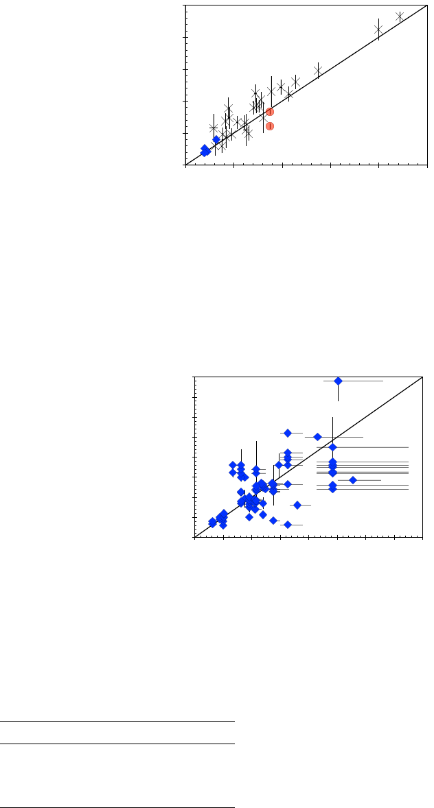
Nova Distances With Gaia DR2 19

10"

15"

20"

25"

0" 5" 10" 15" 20" 25"

Prior""parallax"(mas)"

Gaia"parallax"(mas)"

CV"parallaxes"

Figure 1. Prior parallaxes for novae and cataclysmic variables (CVs). This plot shows the prior parallaxes and the Gaia parallaxes

for four novae (blue diamonds), SS Cyg (red circles), and nearby cataclysmic variables (×s). The diagonal line is to guide the eye for

G a i a

= $

pr i or

. The nova and SS Cyg measures have the prior parallaxes with the HST FGS, and these show real errors that are 3×

larger than their quoted error bars. Despite these problems, the HST parallaxes for just four novae are by far the best distances prior

to Gaia. The ground-based parallaxes from Thorstensen and coworkers for many CVs were made with a 2.4-m telescope, with their

parallaxes having comparable accuracy (i.e., σ

∆µ

) with realistic error bars.

500"

1,000"

1,500"

2,000"

2,500"

3,000"

3,500"

4,000"

0" 500" 1000" 1500" 2000" 2500" 3000" 3500" 4000"

Prior""distance"(pc)"

Gaia"distance"(pc)"

Expansion"parallaxes"

Figure 2. Expansion parallaxes for novae. Prior expansion parallax distances have been published for 22 novae that appear in my Gold

and Silver samples, often with many published widely-varied distances for each nova. As a test of the prior expansion parallaxes, this

plot shows the distances versus the Gaia ground-truth. We see a horrifyingly large scatter. But for the last many decades, expansion

parallaxes were considered as the canonical method.

Table 2. HST FGS parallaxes to four classical novae

Nova $

H ST

(mas) $

G a i a

(mas)

V603 Aql 4.011 ± 0.137 3.191 ± 0.069

DQ Her 2.594 ± 0.207 1.997 ± 0.024

GK Per 2.097 ± 0.116 2.263 ± 0.043

RR Pic 1.920 ± 0.182 1.955 ± 0.030

MNRAS 000, 1–17 (2018)

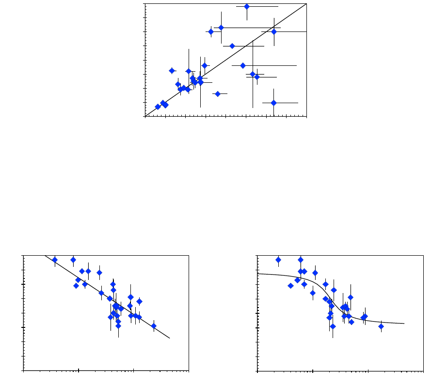
20 B. E. Schaefer

500"

1,000"

1,500"

2,000"

2,500"

3,000"

3,500"

4,000"

0" 500" 1000" 1500" 2000" 2500" 3000" 3500" 4000"

Prior""distance"(pc)"

Gaia"distance"(pc)"

Ex:nc:on"distances"

Ozdonmez"et"al."(2018)"

Figure 3. Testing nova distances based on extinction. The prior nova distances from

Ozd

onmez et al. (2018) are based on many

independent measures of E(B − V ) for each nova, with the extinction as a function of distance along each sightline calibrated with red

clump stars. This exhaustive and consistent work has improved on the earlier hodge-podge of estimates because they are looking closely

at the nova’s line of sight, they used consensus extinction values, and their distances are uniformly evaluated for most novae. This plot

shows a large scatter, but that the extinction-distances are not biased.

-11#

-10#

-9#

-8#

-7#

-6#

-5#

-4#

-3#

1# 10# 100# 1,000#

max

#(mag)#

#(days)#

MMRD#

Downes#&#Duerbeck#(2000)#

max

#vs.#t

-11#

-10#

-9#

-8#

-7#

-6#

-5#

-4#

-3#

1# 10# 100# 1,000#

max

#(mag)#

#(days)#

MMRD#

Downes#&#Duerbeck#(2000)#

max

#vs.#t

Figure 4. The prior MMRD relation. Here, I have plotted the maximum magnitude versus rate of decline relation as given in the

exhaustive Downes & Duerbeck (2000). The maximum magnitude is expressed as the absolute magnitude at peak in the V band, M

ma x

The rate of decline is quantiﬁed by the number of days it takes the nova light curve to decline from peak to 2.0 mag below peak (t

) or

to 3.0 mag below peak (t

). The left panel plots the observed values for t

versus M

ma x

as blue diamonds from Table 5 of Downes &

Durebeck, along with their best ﬁt straight line. The right panel is for the t

version of the relation, along with the four-parameter arctan

function as the best ﬁt. It is this diagram that was used to calibrate the MMRD, as applied over the last two decades. With these plots,

we see that this collection of Milky Way novae do appear to deﬁnitely show the MMRD relation, even though the scatter is huge. That

is, it appears that the faster-fading novae are more luminous.

MNRAS 000, 1–17 (2018)

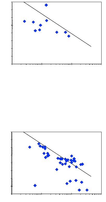
Nova Distances With Gaia DR2 21

-11#

-10#

-9#

-8#

-7#

-6#

-5#

-4#

-3#

1# 10# 100# 1,000#

max

#(mag)#

#(days)#

MMRD#

Recurrent#Novae#

Figure 5. The MMRD for recurrent novae. If we select out the galactic novae for which more than one eruption has been discovered in

the last century or so, then we really expect to get an MMRD similar to the plots in Figure 4. But we see that (1) the RN do not follow

the Downes & Duerbeck MMRD, (2) the scatter is huge about any relation, and (3) there is no signiﬁcant correlation between M

ma x

and t

. This says that the MMRD does not exist for this sample of galactic novae.

-11#

-10#

-9#

-8#

-7#

-6#

-5#

-4#

-3#

1# 10# 100# 1,000#

max

#(mag)#

#(days)#

MMRD#

Gold#+#Silver#samples

Figure 6. The MMRD for the Gold+Silver samples of novae. These 39 novae constitute a test of the MMRD from Downes & Duerbeck

(the black line). The MMRD fails badly. Most of the novae are below the line, so the MMRD relation is greatly biased. Critically, the

scatter is huge, so that the use of any function will return distances that are greatly in error. Thus, the use of the MMRD is bad for any

purpose (individual or statistical) in past or future papers. The scatter is so huge that we have to call into question the very existence

of any MMRD relation (where fast novae are more luminous than slow novae). Nevertheless, a desperate defender of the old ideas can

willfully make a post facto tossing out a quarter of the data, and the remaining points look similar to the large scatter in Figure 4, albeit

with a greatly diﬀerent best-ﬁt equation. So, on the face of it, this plot shows that the MMRD does not apply to galactic novae in any

useful way.

MNRAS 000, 1–17 (2018)

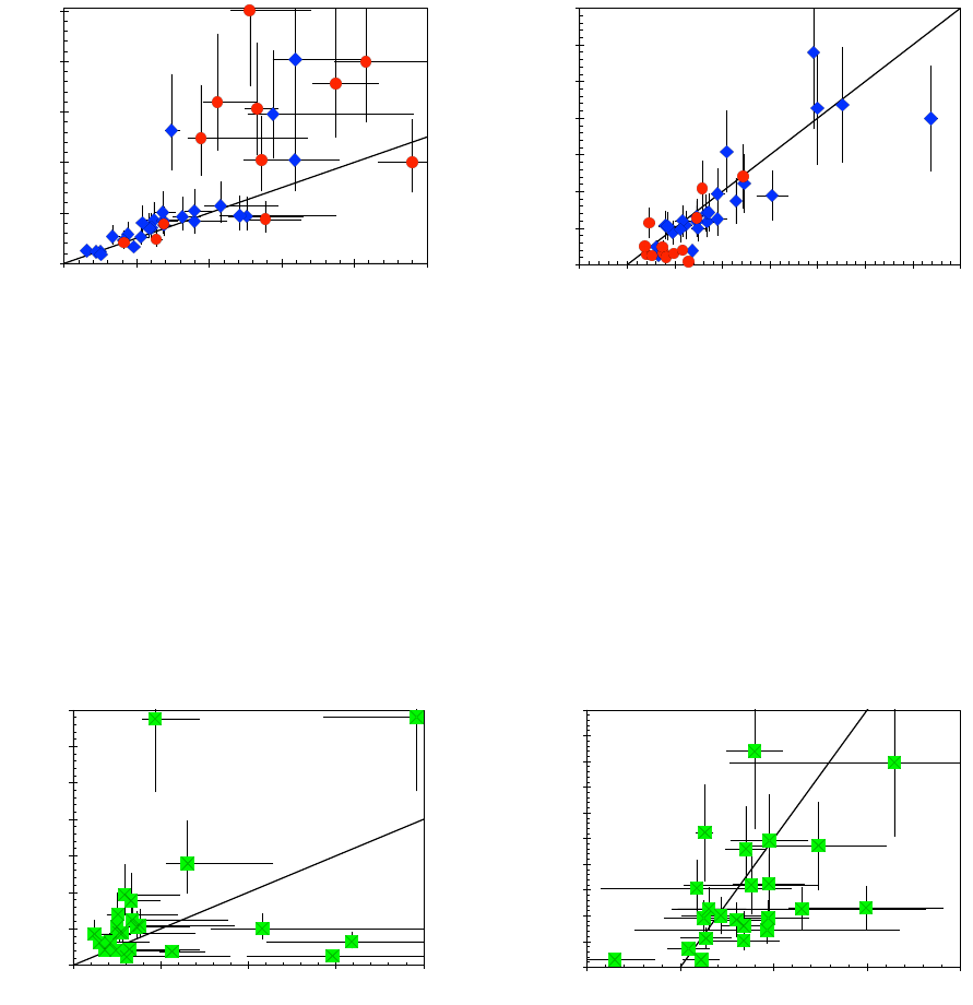
22 B. E. Schaefer

2,000"

4,000"

6,000"

8,000"

10,000"

0" 1000" 2000" 3000" 4000" 5000"

Prior""distance"(pc)"

Gaia"distance"(pc)"

Tes;ng"the"MMRD"

Gold+Silver"samples"

0.0#

0.5#

1.0#

1.5#

2.0#

2.5#

3.0#

3.5#

-0.5# 0.0# 0.5# 1.0# 1.5# 2.0# 2.5# 3.0# 3.5#

Prior##parallax#(mas)#

Gaia#parallax#(mas)#

Tes8ng#the#MMRD#

Gold+Silver#samples#

Figure 7. The distances and parallaxes from the MMRD. These two panels both show the MMRD-derived values for the Gold sample

(blue diamonds) and the Silver sample (red circles). These are essentially the same data as given in Figure 6. The plot of D

pr i or

versus

G a i a

on the left side is an easy way to see the accuracy and errors of the MMRD. If the MMRD is good, then the points should cluster

along the diagonal line to within the plotted 1-sigma error bars. We see immediately that the MMRD has many novae with huge errors.

(Indeed, there is one Silver-sample nova, V721 Sco, that did not ﬁt onto the plot for any useful range, being at D

pr i or

=24100

+10300

−7200

and D

G a i a

=1570

+160

−100

pc.) We see 8 out of 39 novae have >2× errors in distance (or >4× in luminosity). Further, with 29 out of 39 novae

having D

pr i or

> D

G a i a

, we see that the old MMRD has a large systematic bias. Another way of looking at these same data is to plot

pr i or

versus $

G a i a

, as in the panel on the right. Again we see that most of the novae are below the $

pr i or

= $

G a i a

line (shown

as the black diagonal line), many of the points deviate by more than a factor of two from the diagonal line, and 46% of the novae are

>1-sigma from the line. All this goes to show that the MMRD is too poor in accuracy to use for individual novae or to use for statistical

purposes.

5,000"

10,000"

15,000"

20,000"

25,000"

30,000"

35,000"

0" 5000" 10000" 15000" 20000"

Prior""distance"(pc)"

Gaia"distance"(pc)"

Tes8ng"the"MMRD"

Bronze"sample"

0.0#

0.1#

0.2#

0.3#

0.4#

0.5#

0.6#

0.7#

0.8#

0.9#

1.0#

-0.5# 0.0# 0.5# 1.0# 1.5#

Prior##parallax#(mas)#

Gaia#parallax#(mas)#

Tes=ng#the#MMRD#

Bronze#sample#

Figure 8. Testing the MMRD with the Bronze sample. The Bronze sample includes 23 novae for which the fractional error in the Gaia

parallax is >30%, and so the distances have large error bars. The left-side panel gives D

pr i or

versus D

G a i a

, while the right-side panel

gives $

pr i or

versus $

G a i a

. In an ideal world, the points would be tightly clustered around the D

pr i or

G a i a

diagonal line. What

we see is a huge scatter. This conﬁrms the conclusions from Figure 7. However, in this ﬁgure, the error bars are suﬃciently large that we

cannot use the Bronze sample alone to convict the MMRD of failure.

MNRAS 000, 1–17 (2018)

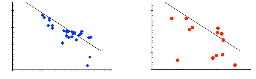
Nova Distances With Gaia DR2 23

-11#

-10#

-9#

-8#

-7#

-6#

-5#

-4#

-3#

1# 10# 100# 1,000#

max

#(mag)#

#(days)#

MMRD#

Gold#sample

-11#

-10#

-9#

-8#

-7#

-6#

-5#

-4#

-3#

1# 10# 100# 1,000#

max

#(mag)#

#(days)#

MMRD#

Silver#sample

Figure 9. The MMRD for the Gold and Silver samples separately. These two plots show the MMRD for the Gold sample (the panel

on the left) and the Silver sample (the panel on the right). Both of these plots can be directly compared to Figure 4a, with the same

range and scale for both axes, and with the MMRD relation from Downes & Duerbeck (solid black line). We see that the Gold sample

does display an apparent relation between M

ma x

and t

, but there is huge scatter including several far outliers, and the best ﬁt relation

is substantially diﬀerent from the pre-Gaia relation. So if we willfully paid attention only to the Gold sample, then we could continue

the old faith that we can pull out some utility from the MMRD. But the Silver sample shows no relation at all between M

ma x

and t

Rather, we see much of the diagram ﬁlled in, so the existence of the MMRD is denied. The utter failure of the MMRD as shown in the

Silver sample is also shown for novae in M31, for novae in M87, for galactic recurrent novae, and for grids of theoretical models of novae.

So we are faced with the dilemma of reconciling the two panels in this ﬁgure, where the Gold sample shows a real MMRD relation (albeit

with so much scatter as to be essentially useless) while the Silver sample denies the existence of any MMRD.

MNRAS 000, 1–17 (2018)

24 B. E. Schaefer

Table 3. Published Expansion Parallaxes Compared to Gaia

Nova D

G a i a

(pc) D

pr i or

(pc)

V603 Aql 314

−7

330, 400

V1494 Aql 1239

+422

−127

1200

T Aur 880

+46

−35

960±220, 1500

V705 Cas 2157

+799

−228

2500

V842 Cen 1379

+120

−78

420, 1200, 1140, 1150, 1300±500, 1325

V476 Cyg 665

+107

−53

1620±120, 1800

V1974 Cyg 1631

+261

−131

310, 1320, 1800±100, 1940, 2000, 2115,

∼2600

HR Del 958

+35

−29

505, 750, 760±130, 825, 900, 940±155,

1010

DQ Her 501

−6

300, 400±60, 480±50, 560±20

V446 Her 1361

+185

−100

1350

V533 Her 1202

+52

−41

560±70, 850±150, 1250±30, 1300, 1320

CP Lac 1170

+67

−50

1350

DK Lac 2517

+788

−261

3900±500

BT Mon 1477

+128

−84

1800±300

GK Per 442

−8

455±30, 500

RR Pic 511

−8

500, 580, 600±60

CP Pup 814

+15

−14

850, 900, 1120, 1140, 1500, 1600, 1700,

1800±400

FH Ser 1060

+112

−68

700, 850±50, 870±90, 920±130, 950±50

V382 Vel 1800

+243

−133

800

NQ Vul 1080

+169

−85

910, 1160±210, 1200, 1280, 1600±800,

1700

PW Vul 2420

+1337

−277

1200, 1300, 1500-3000, 1600, 1635, 1750,

1800±50, 1880

CT Ser 2774

+495

−268

1430

Table 4. Collected results for quality of prior nova distances

Prior Method Nova Sample N

no v a

∆µ

h∆µi

HST FGS parallaxes Harrison et al. (2013) 4 0.37 3.03 -0.21

Ground-based parallaxes CVs of Thorstensen 26 0.54 1.06 -0.37

Expansion parallaxes Slavin (1997) 9 1.04 3.60 -0.10

Expansion parallaxes Table 3 75 0.95

-0.06

Blackbody distance to secondary V1017 Sgr (Salazar et al. 2016) 1 ... χ=-0.14 -0.05

Reddening-distance relation

Ozd

onmez et al. (2016) 15 1.32 4.25 -0.05

Reddening-distance relation

Ozd

onmez et al. (2018) 5 1.01 1.31 0.12

RDR and parallaxes

Ozd

onmez et al. (2018) 28 1.15 2.45 -0.05

MMRD for t

Gold+Silver 39 1.31 1.03 0.73

MMRD for t

Gold 26 0.82 0.83 0.43

MMRD for t

Silver 13 1.85 1.32 1.32

MMRD for t

Bronze 23 2.20 1.68 0.44

15d

= -5.23±0.39 mag Gold+Silver 34 1.53 2.26 0.04

15d

= -5.23±0.39 mag Gold+Silver (t

>10 days) 23 1.08 2.21 -0.28

ma x

= -7.0±1.4 mag Gold+Silver 37 1.61

0.00

Nova light echo T Pyx (Sokoloski et al. 2013) 1 ... χ=2.05 0.89

Combining multiple methods Schaefer papers 5 0.93 0.86 0.82

Combining multiple methods Duerbeck (1981) 17 1.05 4.38 -0.43

Combining multiple methods Patterson (1984) 9 0.42

0.04

Combining multiple methods Patterson et al. (2013) 13 0.44

0.17

Theory models Hachisu & Kato papers 16 0.76 1.66 0.16

Formal uncertainties are not available for most novae in the

set.

The ±1.4 value was chosen so that σ

=1.00.

MNRAS 000, 1–17 (2018)